Step 3: Fitting Peaks

Notebook Code: Notebook Prose:

The meat of hplc-py is its ability to take in windowed regions of a chromatogram and fit a number of peaks such that the chromatogram in that region is well reconstructed. As is the theme in these notebooks, it’s easier to look at a chromatogram and see what the reconstituted signals should like than to do it quantitatively.

Ideally, one would have a physical model that would describe how an analyte interacts with the stationary phase of the chromatography column and a generative model that would capture the statistical distribution of the measurements as a function of time. However, having this in chromatography is exceedingly rare, so we are left with phenomenological descriptions of peak shape that we relate to chemical species and concentrations through calibration curves and control experiments. This is what hplc-py excels at–phenomenological quantitative description of signals in a chromatogram. It is important to note that hplc-py does not provide a model of the components of the chromatogram but rather fits the parameters of a minimal number of convolved signals that can capture the observed data in the chromatogram. In this notebook, we outline how this fitting procedure is executed and how the total chromatographic signal is reconstructed.

The Skew-Normal Distribution

In hplc-py, we consider that each detected maximum in a chromatogram results from a single compound \(i\) whose time-dependent signal intensity \(S_i\) can be phenomenologically well described by an amplitude-weighted skew normal distribution. Mathematically, this is defined as

\[S_i(t) = \frac{A}{\sqrt{2\pi\sigma_i^2}} \exp\left[\frac{(t - \tau_i)^2}{2\sigma_i^2}\right]\left[1 + \text{erf}\left(\frac{\alpha_i (t - \tau_i)}{\sqrt{2\sigma^2}}\right)\right], \tag{1}\]

where \(\text{erf}\) is the error function, \(A\) is the amplitude, \(\tau\) is the retention time, \(\sigma^2\) is the signal variance, and \(\alpha\) is the skew parameter. The skew normal distribution is used because the skew parameter \(\alpha\) can break symmetry, allowing for heavily tailed signals. When the distribution is unskewed, meaning \(\alpha = 0\), Eq. 1 simplifies to a Normal distribution symmetric about \(\tau\). To get a sense of how \(\alpha\) impacts the resulting signal, we can use scipy.stats.skewnormal to examine the amplitude-weighted output,

[1]:

import numpy as np
import pandas as pd
import scipy.stats
import matplotlib.pyplot as plt
import seaborn as sns
sns.set()

# Set a range of skew parameters to demonstrate the signal as a function of time
alpha_range = [-5, -1, 0, 1, 5]
time = np.arange(0, 20, 0.01 )

# Set constants for each signal
A = 100
tau = 10
sigma = 3
for alpha in alpha_range:
    # Compute the skew normal distribution and plot the resulting signal.
    signal = A * scipy.stats.skewnorm(alpha, loc=tau, scale=sigma).pdf(time)
    plt.plot(time, signal, label=alpha, lw=2)

# Add necessary labels
plt.xlabel('time')
plt.ylabel('$S$')
plt.legend(title=r'$\alpha$')

[1]:

<matplotlib.legend.Legend at 0x1788ded40>

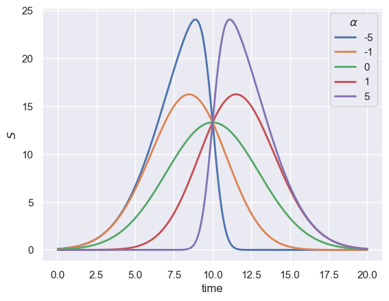
When the skew parameter \(\alpha\) is large and negative, the signal is heavily skewed towards shorter retention times. Even though all signals in this plot have different heights and locations of the maxima, they all have identical values for \(A\), \(\tau\), and \(\sigma\). The flexibility of \(\alpha\) in defining the signal trace allows for a broad array of peak shapes to be well described by this distribution.

Fitting Peak Windows

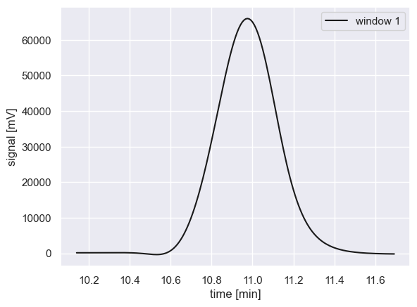
As described in the notebook for Step 2, a chromatogram is broken down into multiple “peak windows” which likely contain overlapping analyte signals. Each window is fitted independently, which assumes that distant peaks have no influence on each other. As an example, let’s look at a real peak window from a sample chromatogram.

[2]:

from hplc.quant import Chromatogram
import pandas as pd

# Load an example chromatogram and correct the baseline
df = pd.read_csv('data/sample_chromatogram.txt')
chrom  = Chromatogram(df, cols={'time':'time_min', 'signal':'intensity_mV'},
                      time_window=[10, 20])
chrom.correct_baseline()

# Assign the peak windows with a modified buffer and prominence filter
windows = chrom._assign_windows(buffer=50, prominence=0.01)

# Get the first peak window and plot
first_peak = windows[(windows['window_type']=='peak') & (windows['window_id']==1)]
plt.plot(first_peak['time_min'], first_peak['intensity_mV_corrected'], 'k-', label='window 1')
plt.xlabel('time [min]')
plt.ylabel('signal [mV]')
plt.legend()

Performing baseline correction: 100%|██████████| 299/299 [00:00<00:00, 3935.20it/s]

[2]:

<matplotlib.legend.Legend at 0x1789c3280>

To determine the properties of this peak (including its area which is proportional to concentration), we will find the best-fit parameters using a non-linear least squares trust region fitting method as is implemented in scipy.optimize.curve_fit which is a robust estimation algorithm for bounded problems.

To do so, we must provide i) initial guesses for the parameters \([A, \tau, \sigma, \alpha]\) and ii) reasonable bounds on their values.

Default settings for initial guesses of parameters

In hplc-py, initial guesses are set given the properties of the observed chromatogram. These default parameter guesses are:

\(A_0 \rightarrow\) the observed value of the chromatogram at the location of the maxima
\(\tau_0 \rightarrow\) the observed time-location of the maxima
\(\sigma_0 \rightarrow\) one-half of the observed peak width at its half-maximal value
\(\alpha_0 \rightarrow\) 0, which guesses that the peak is approximately Gaussian.

These values are determined using peak measurements returned by scipy.signal.find_peaks and scipy.signal.peak_widths. These properties are accessible via the chromatogram attribute .window_props

[3]:

# Set the initial guesses from the window properties
props = chrom.window_props[1]
p0 = [props['amplitude'][0],
     props['location'][0],
     props['width'][0] / 2,
     0]
p0

[3]:

[65992.999952423, 10.98, 0.16630057317687066, 0]

Default bounds for parameters

By default, hplc-py applies broad, permissive bounds on these parameters given information of the chromatogram. The default bounds given to each parameter are

\(A \in [0.1 \times A_0, 10 \times A_0]\) where \(A_0\) is the initial guess for the amplitude.
\(\tau \in [t_{min}, t_{max}]\) where \(t_{min}\) and \(t_{max}\) correspond to the minimum and maximum times in the peak window.
\(\sigma_{bounds} \in [dt, \frac{t_{max} - t_{min}}{2}]\) where \(dt\) corresponds to the time sampling interval of the chromatogram.
\(\alpha \in (-\inf, +\inf)\).

These bounds can be overridden for all peak inferences by providing a dictionary of their values, as is specified in the documentation for hplc.quant.Chromatogram.fit_peaks.

[4]:

# Give initial bounds for the parameters (lower, upper)
bounds = [[], []]
bounds[0] = [p0[0] * 0.1, first_peak['time_min'].min(), chrom._dt, -np.inf]
bounds[1] = [p0[0] * 10, first_peak['time_min'].max(), 0.5 * (first_peak['time_min'].max() - first_peak['time_min'].min()), np.inf]

Optimization of parameters

Given initial guesses and parameter bounds, the best-fit parameters are estimated by calling scipy.optimize.curve_fit on the observed data in the peak widow. The cost function is defined as a method _fit_skewnorms of a Chromatogram.

[5]:

import scipy.optimize

# Perform the fit
param_opt, _ = scipy.optimize.curve_fit(chrom._fit_skewnorms, first_peak['time_min'],
                                        first_peak['intensity_mV_corrected'],
                                        p0=p0, bounds=bounds)
print(f'Optimal parameters (amplitude, location, scale, skew) : {param_opt}')

Optimal parameters (amplitude, location, scale, skew) : [2.33773945e+04 1.09020036e+01 1.59217385e-01 7.03685471e-01]

With the optimal parameters estimated, we can compare the inferred signal to the observed chromatogram

[6]:

# Compute the amplitude-weighted skewnorm with the inferred parameters
fit = param_opt[0] * scipy.stats.skewnorm(param_opt[3], loc=param_opt[1], scale=param_opt[2]).pdf(first_peak['time_min'])

# Plot the data and the observed peak
plt.plot(first_peak['time_min'], first_peak['intensity_mV_corrected'], 'k-', label='window 1')
plt.fill_between(first_peak['time_min'], fit, color='dodgerblue', label='inferred signal')
plt.xlabel('time [min]')
plt.ylabel('signal [mV]')
plt.legend()

[6]:

<matplotlib.legend.Legend at 0x178c7f7c0>

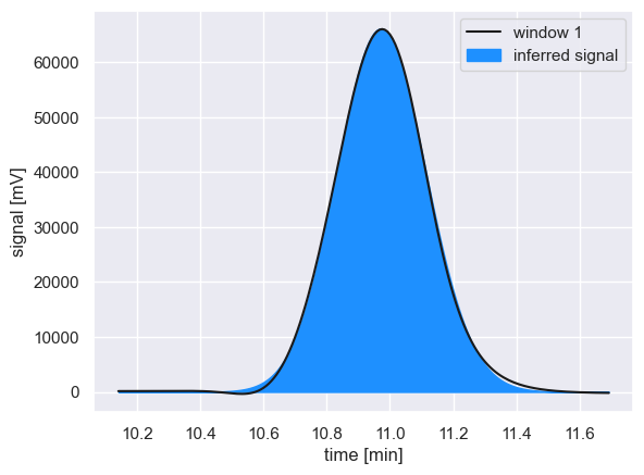
With an adequate reconstruction of the observed peak, the signal area is computed by integrating the signal over the entire time range of the peak window, and the procedure is repeated for the next peak window.