Quickstart

Notebook Code: Notebook Prose:

This package is meant to get you from chromatogram to quantified peaks as rapidly as possible. Below is a brief example of how to go from a raw, off-the-machine data set to a list of compounds and their absolute concentrations.

Loading and viewing chromatograms

Text files containing chromatograms with time and signal information can be intelligently read into a pandas DataFrame using hplc.io.load_chromatogram().

[43]:

# Load the chromatogram as a dataframe
from hplc.io import load_chromatogram
df = load_chromatogram('data/sample.txt',
                                 cols=['R.Time (min)', 'Intensity'])
df.head()

[43]:

	R.Time (min)	Intensity
0	0.00000	0
1	0.00833	0
2	0.01667	0
3	0.02500	0
4	0.03333	-1

By providing the column names as a dictionary, you can rename the (often annoying) default column names to something easier to work with, such as “time” and “signal” as

[44]:

# Load chromatogram and rename the columns
df = load_chromatogram('data/sample.txt', cols={'R.Time (min)':'time',
                                                              'Intensity': 'signal'})
df.head()

[44]:

	time	signal
0	0.00000	0
1	0.00833	0
2	0.01667	0
3	0.02500	0
4	0.03333	-1

This dataframe can now be loaded passed to the Chromatogram class, which has a variety of methods for quantification, cropping, and visualization and more.

[45]:

# Instantiate the Chromatogram class with the loaded chromatogram.
from hplc.quant import Chromatogram
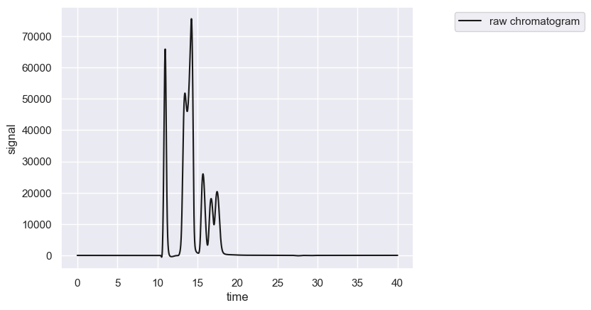
chrom = Chromatogram(df)

# Show the chromatogram
chrom.show()

[45]:

[<Figure size 640x480 with 1 Axes>, <Axes: xlabel='time', ylabel='signal'>]

The crop method allows you to crop the chromatogram in place to restrict the signal to a specific time range.

[47]:

# Crop the chromatogram in place between 8 and 21 min.
chrom.crop([10, 20])
chrom.show()

[47]:

[<Figure size 640x480 with 1 Axes>, <Axes: xlabel='time', ylabel='signal'>]

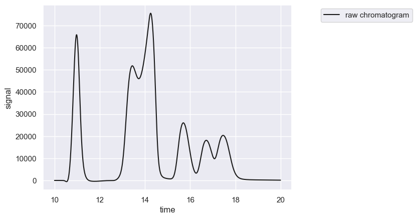
Note that the crop function operates in place and modifies the loaded as data within the Chromatogram object.

Detecting and Fitting Peaks

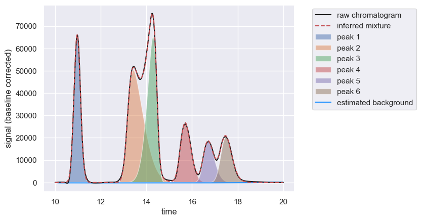
The real meat of the package comes in the deconvolution of signal into discrete peaks and measurement of their properties. This typically involves the automated estimation and subtraction of the baseline, detection of peaks, and fitting of skew-normal distributions to reconstitute the signal. Luckily for you, all of this is done in a single method call Chromatogram.fit_peaks()

[49]:

# Automatically detect and fit the peaks
peaks = chrom.fit_peaks(buffer=0)
peaks

Performing baseline correction: 100%|██████████| 299/299 [00:00<00:00, 3464.65it/s]
Deconvolving mixture: 100%|██████████| 2/2 [00:00<00:00,  6.73it/s]

[49]:

retention_time	scale	skew	amplitude	area	peak_id
10.90	0.158762	0.691800	23380.461934	2.805655e+06	1
13.17	0.594750	3.905677	43165.789520	5.179895e+06	2
14.45	0.349607	-2.995704	34697.471686	4.163697e+06	3
15.53	0.314009	1.621208	15061.835818	1.807420e+06	4
16.52	0.347376	1.991205	10939.067960	1.312688e+06	5
17.29	0.348123	1.705571	12525.991656	1.503119e+06	6

To see how well the deconvolution worked, you can once again call the show method to see the composite compound chromatograms.

[40]:

# View the result of the fitting.
chrom.show()

[40]:

[<Figure size 640x480 with 1 Axes>,
 <Axes: xlabel='time', ylabel='signal (baseline corrected)'>]

../_images/tutorials_quickstart_15_1.png

You can also call assess_fit() to see how well the chromatogram is described by the inferred mixture. This is done through computing a reconstruction score \(R\) defined as

\[R = \frac{\text{Area estimated through inference} + 1}{\text{Area observed in signal} + 1}.\]

This is computed for regions with peaks (termed “peak windows”) and regions of background (termed “interpeak windows”) if they are present.

[41]:

# Print out the assessment statistics.
scores = chrom.assess_fit()
scores.head()


-------------------Chromatogram Reconstruction Report Card----------------------

Reconstruction of Peaks
=======================

A+, Success:  Peak Window 1 (t: 2.910 - 17.460) R-Score = 1.0000

Signal Reconstruction of Interpeak Windows
==========================================

A+, Success:  Interpeak Window 1 (t: 0.000 - 2.900) R-Score = 1.0000 & Fano Ratio = 0
A+, Success:  Interpeak Window 2 (t: 17.470 - 19.990) R-Score = 1.0000 & Fano Ratio = 0

--------------------------------------------------------------------------------

[41]:

	window_id	time_start	time_end	signal_area	inferred_area	signal_variance	signal_mean	signal_fano_factor	reconstruction_score	window_type	applied_tolerance	status
0	1	0.00	2.90	1.0	1.000000	0.00000	1.000000e-09	0.000000	1.000000	interpeak	0.01	valid
1	2	17.47	19.99	1.0	1.000000	0.00000	1.000000e-09	0.000000	1.000000	interpeak	0.01	valid
0	1	2.91	17.46	12001.0	12001.463355	204.39806	8.241758e+00	24.800298	1.000039	peak	0.01	valid

Quantifying Peaks

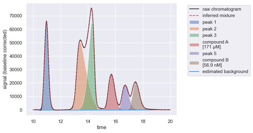
If you know the parameters of the linear calibration curve, which relates peak area to a known concentration, you can use the map_compounds method which will map user provided compound names to peaks.

[11]:

# Define the two peaks of interest and their calibration curves
calibration = {'compound A': {'retention_time': 15.5,
                              'slope': 10547.6,
                              'intercept': -205.6,
                              'unit': 'µM'},
               'compound B': {'retention_time': 17.2,
                              'slope': 26401.2,
                              'intercept': 54.2,
                              'unit': 'nM'}}
quant_peaks = chrom.map_peaks(calibration)
quant_peaks

[11]:

	retention_time	scale	skew	amplitude	area	peak_id	compound	concentration	unit
0	15.53	0.314009	1.621208	15061.835818	1.807420e+06	4	compound A	171.377934	µM
0	17.29	0.348123	1.705571	12525.991656	1.503119e+06	6	compound B	56.931685	nM

Successfully mapping compounds to peak ID’s will also be reflected in the show method.

[13]:

# Show the chromatogram with mapped compounds
chrom.show()

[13]:

[<Figure size 640x480 with 1 Axes>,
 <Axes: xlabel='time', ylabel='signal (baseline corrected)'>]

../_images/tutorials_quickstart_22_1.png

Deconvolving Overlapping and Subtle Peaks

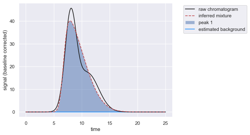
Often, compounds will have similar retention times leading to heavily overlapping peaks. If one of the compounds dominates the signal, the other compounds may only show up as a “shoulder” on the predominant peak. In this case, automatic peak detection will fail and will fit only a single peak, as in the following example.

[15]:

# Load, fit, and display a chromatogram with heavily overlapping peaks
df = load_chromatogram('data/example_overlap.txt', cols=['time', 'signal'])
chrom = Chromatogram(df)
peaks = chrom.fit_peaks()
chrom.show()
score = chrom.assess_fit()

Performing baseline correction: 100%|██████████| 249/249 [00:00<00:00, 1499.35it/s]
Deconvolving mixture: 100%|██████████| 1/1 [00:00<00:00, 99.62it/s]


-------------------Chromatogram Reconstruction Report Card----------------------

Reconstruction of Peaks
=======================

F, Failed:  Peak Window 1 (t: 1.810 - 21.090) R-Score = 0.9788
Peak mixture poorly reconstructs signal. You many need to adjust parameter bounds
or add manual peak positions (if you have a shouldered pair, for example). If
you have a very noisy signal, you may need to increase the reconstruction
tolerance `rtol`.

Signal Reconstruction of Interpeak Windows
==========================================

A+, Success:  Interpeak Window 1 (t: 0.000 - 1.800) R-Score = 0.9963 & Fano Ratio = 10^-5
C-, Needs Review:  Interpeak Window 2 (t: 21.100 - 24.990) R-Score = 1.2596 & Fano Ratio = 0
Interpeak window 2 is not well reconstructed by mixture, but has a small Fano factor
compared to peak region(s). This is likely acceptable, but visually check this region.


--------------------------------------------------------------------------------

../_images/tutorials_quickstart_24_2.png

However, if you know there is a second peak, and you know its approximate retention time, you can manually add an approximate peak position, forcing the algorithm to estimate the peak convolution including more than one peak.

[16]:

# Enforce a manual peak position at around 11 time units
peaks = chrom.fit_peaks(known_peaks=[12])
chrom.show()
score = chrom.assess_fit()

Deconvolving mixture: 100%|██████████| 1/1 [00:00<00:00,  2.92it/s]


-------------------Chromatogram Reconstruction Report Card----------------------

Reconstruction of Peaks
=======================

A+, Success:  Peak Window 1 (t: 1.810 - 21.090) R-Score = 1.0000

Signal Reconstruction of Interpeak Windows
==========================================

A+, Success:  Interpeak Window 1 (t: 0.000 - 1.800) R-Score = 1.0145 & Fano Ratio = 10^-5
A+, Success:  Interpeak Window 2 (t: 21.100 - 24.990) R-Score = 1.0019 & Fano Ratio = 0

--------------------------------------------------------------------------------

../_images/tutorials_quickstart_26_2.png

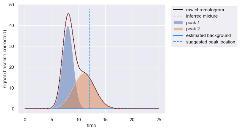
Note that even though we provided a guess of ≈ 12 time units for the position of the second peak, the algorithm did not force the peak to be exactly there. If enforced_locations are provided, these are used as initial guesses when performing the fitting.

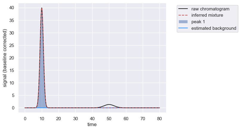
This approach can also be used if there is a shallow, isolated peak that is not automatically detected.

[17]:

# Load and fit a sample with a shallow peak
df = load_chromatogram('data/example_shallow.csv', cols=['time', 'signal'])
chrom = Chromatogram(df)
peaks = chrom.fit_peaks(prominence=0.5) # Prominence is to exclude shallow peak
chrom.show()
score = chrom.assess_fit()

Performing baseline correction:   0%|          | 0/249 [00:00<?, ?it/s]

Performing baseline correction: 100%|██████████| 249/249 [00:00<00:00, 461.48it/s]
Deconvolving mixture: 100%|██████████| 1/1 [00:00<00:00, 10.76it/s]


-------------------Chromatogram Reconstruction Report Card----------------------

Reconstruction of Peaks
=======================

A+, Success:  Peak Window 1 (t: 2.910 - 17.080) R-Score = 1.0000

Signal Reconstruction of Interpeak Windows
==========================================

A+, Success:  Interpeak Window 1 (t: 0.000 - 2.900) R-Score = 1.0000 & Fano Ratio = 0
F, Failed:  Interpeak Window 2 (t: 17.090 - 79.990) R-Score = 10^-3 & Fano Ratio = 0.0369
Interpeak window 2 is not well reconstructed by mixture and has an appreciable Fano
factor compared to peak region(s). This suggests you have missed a peak in this
region. Consider adding manual peak positioning by passing `known_peaks`
to `fit_peaks()`.

--------------------------------------------------------------------------------

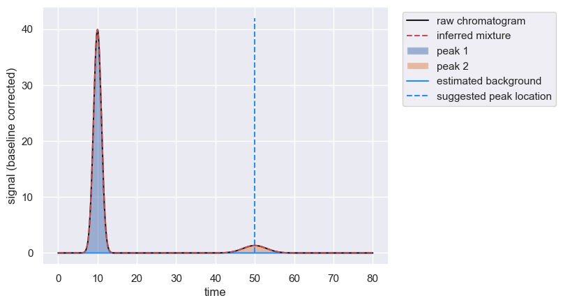
../_images/tutorials_quickstart_29_3.png

As the second peak is broad, you can provide an estimate of the width of the peak at the half maximum value to provide a better initial guess.

[18]:

# Add the location of the second peak
peaks = chrom.fit_peaks(known_peaks={50 : {'width': 5}}, prominence=0.5)
chrom.show()
score = chrom.assess_fit()

Deconvolving mixture: 100%|██████████| 2/2 [00:00<00:00, 17.89it/s]


-------------------Chromatogram Reconstruction Report Card----------------------

Reconstruction of Peaks
=======================

A+, Success:  Peak Window 1 (t: 2.910 - 17.080) R-Score = 1.0000
A+, Success:  Peak Window 2 (t: 45.000 - 54.990) R-Score = 1.0000

Signal Reconstruction of Interpeak Windows
==========================================

A+, Success:  Interpeak Window 1 (t: 0.000 - 2.900) R-Score = 1.0000 & Fano Ratio = 0
A+, Success:  Interpeak Window 2 (t: 17.090 - 44.990) R-Score = 1.0016 & Fano Ratio = 0.0154
A+, Success:  Interpeak Window 3 (t: 55.000 - 79.990) R-Score = 1.0002 & Fano Ratio = 0.0153

--------------------------------------------------------------------------------

../_images/tutorials_quickstart_31_2.png

Constraining Peaks With Known Parameters

If you have a chromatogram with two completely overlapping peaks, it can be very, very difficult to deconvolve the mixture. However, if you happen to know the parameters of one of the constituents (say, from characterization of an isolated aqueous mixture of that compound), you can apply more stringent bounds to that particular peak. Say for example we have a mixture of two compounds with retention times of 10 and 10.6 and you know that the first peak has an amplitude of 100 units. If you were to only supply the locations of the known peaks, you would underestimate the contribution from the first peak.

[19]:

# Load a chromatogram that is very heavily overlapping
df = load_chromatogram('data/bounding_example.csv', cols=['time', 'signal'])
chrom = Chromatogram(df)

# Fit the peaks providing only the known retention times
peaks = chrom.fit_peaks(known_peaks = [10, 10.6])
inferred_amplitude = peaks[peaks['peak_id']==1]['amplitude'].values[0]
known_amplitude = 100

# Print a summary statement demonstrating the underestimation
print(f'Inferred amplitude for peak 1 is {inferred_amplitude:0.3f}. Known value is {known_amplitude:0.3f}')
chrom.show()

Performing baseline correction: 100%|██████████| 249/249 [00:00<00:00, 1365.51it/s]
Deconvolving mixture: 100%|██████████| 2/2 [00:00<00:00, 14.02it/s]

Inferred amplitude for peak 1 is 94.971. Known value is 100.000

[19]:

[<Figure size 640x480 with 1 Axes>,
 <Axes: xlabel='time', ylabel='signal (baseline corrected)'>]

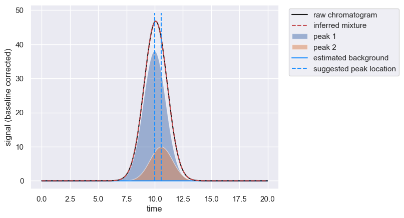
../_images/tutorials_quickstart_33_4.png

You can constrain the parameter bounds for the amplitude of peak 1 more narrowly than the other peak by passing a dictionary to the known_peaks parameter of fit_peaks().

[20]:

# Define more stringent bounds as a dictionary with the retention time as the key
# and the parameter bounds as a value.
bounds = {10: {'amplitude':[99, 101]}, # Known parameters for peak 1
          10.6 : {} # Allow free inference for second peak
          }
peaks = chrom.fit_peaks(known_peaks=bounds)
inferred_amplitude = peaks[peaks['peak_id']==1]['amplitude'].values[0]

# Print a summary statement demonstrating the improvement.
print(f'Inferred amplitude for peak 1 is {inferred_amplitude:0.3f}. Known value is {known_amplitude:0.3f}')
chrom.show()

Deconvolving mixture:   0%|          | 0/2 [00:00<?, ?it/s]

Deconvolving mixture: 100%|██████████| 2/2 [00:00<00:00,  2.08it/s]

Inferred amplitude for peak 1 is 99.000. Known value is 100.000

[20]:

[<Figure size 640x480 with 1 Axes>,
 <Axes: xlabel='time', ylabel='signal (baseline corrected)'>]

../_images/tutorials_quickstart_35_5.png

Here, we’ve only bounded the amplitude parameter, but you can also provide bounds for location, scale, and skew.