Step 4: Scoring the Reconstruction

Notebook Code: Notebook Prose:

After estimation and subtraction of the baseline, detection of peaks, splitting into windows, and fitting the peaks to a phenomenological function, we are left with the irritating problem of assessing how well we have done. Consider the following chromatogram:

[1]:

from hplc.quant import Chromatogram
import pandas as pd

# Load the sample chromatogram and fit the peaks using default parameters.
df = pd.read_csv('data/sample_chromatogram.txt')
chrom = Chromatogram(df, cols={'time':'time_min', 'signal':'intensity_mV'},
                     time_window=[10, 20])
peaks = chrom.fit_peaks()
chrom.show()

Performing baseline correction: 100%|██████████| 299/299 [00:00<00:00, 3977.22it/s]
Deconvolving mixture: 100%|██████████| 2/2 [00:10<00:00,  5.20s/it]

[1]:

[<Figure size 640x480 with 1 Axes>,
 <Axes: xlabel='time_min', ylabel='intensity_mV (baseline corrected)'>]

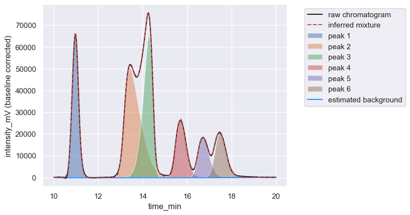
By eye, this looks like a very good reconstruction of the chromatogram, but it would be nice to have a quantitative measure.

The Reconstruction Score

Quantifying concentrations from HPLC data requires a measure of the Area Under the Curve (AUC), or more correctly stated, the integrated signal over a given time interval. A perfect reconstruction of the chromatogram, resulting from summing over all constituent peaks in a mixture, would yield an identical AUC over any given time interval as the integrated signal of the original chromatogram. This can be defined mathematically as

\[\frac{\sum\limits_i^{N_\text{peaks}} \sum\limits_{t=0}^{t_\text{max}}S_i(t)}{\sum\limits_{t=0}^{t_\text{max}}S(t)^\text{(observed)}} = \frac{\text{AUC}^\text{(inferred)}}{\text{AUC}^\text{(observed)}} = 1, \tag{1}\]

where \(i\) represents the \(i\)-th component signal, \(N_\text{peaks}\) denotes the number of peaks in a given peak window, and \(t\) denotes the discrete time point. In peak windows where the constituent signal is very small \(S_{i}^\text{(observed)} \rightarrow 0\), even small deviations between the inferred mixture and the observed signal can cause this quantity to be much larger or much smaller than one, even if the total integrated signal difference is small.

To account for this fact, we can modify Eq. 1 as

\[R = \frac{1 + \text{AUC}^\text{(inferred)}}{1 + \text{AUC}^{(observed)}}, \tag{2}\]

which we term a reconstruction score or \(R\)-score for short.

In practice, you’ll never get an \(R\)-score of exactly 1, but you can get close. For example, an \(R\)-score can be computed for the chromatogram reconstruction shown above by calling the _score_reconstruction method of a Chromatogram object:

[2]:

# Compute the R_score for the above chromatogram
scores = chrom._score_reconstruction()
scores[['window_type', 'window_id', 'reconstruction_score']]

[2]:

	window_type	window_id	reconstruction_score
0	peak	1	0.997252
1	peak	2	0.995222
0	interpeak	1	0.390152
1	interpeak	2	0.000200
2	interpeak	3	0.084916

For the two peak windows (rows 1 & 2), the \(R\)-score is very close to one, within 0.01. Whether that is sufficient for your case or not is up to you, dear reader. My job is just to give you that number.

Scoring the regions between peaks

But what about the interpeak regions? These windows correspond to the chromatogram signal that lies outside of peak windows – thus, an \(R\)-score is a measure of how well you are reconstructing the subtracted baseline. As there will almost always be 0 inferred signal in this region, your \(R\)-scores will typically be terrible and close to 0.

While this will usually mean you are just not reconstructing the signal noise, a terrible \(R\)-score in an interpeak region may mean that there are peaks present, but your choice of a prominence filter is not detecting them. In this case, it is better to have a measure of what the noise-to-signal ratio is in these regions.

Mathematically, we can compute this as the Fano factor of the region, which can be thought of as a measure of the “predictability” of the signal in this sequence. This can be computed as

\[F = \frac{\langle S^2 \rangle - \langle S \rangle^2}{\langle S \rangle}, \tag{3}\]

where \(S\) is the signal within a peak window. If the Fano factor is small, then the region is likely background noise whereas a large Fano factor would indicate there may be a peak present and you need to adjust your peak detection criteria.

But what determines if it’s big or small? As all chromatograms have a peak (why else would you be using hplc-py?), we can compare the Fano factor of the interpeak regions to the average Fano factors of the regions where we know there is signal. If this quantity, which term the Fano ratio, is close to zero, then it is likely the interpeak region is just noise and you are not missing anything substantive. However, if the Fano ratio is not close to zero, there may be a peak present. Again, what determines “close” to zero is arbitrary.

Generating a chromatogram report card

In hplc-py, you can automatically generate “report” cards by calling the assess_fit method of a Chromatogram object. For the chromatogram above, the report card looks pretty good!

[3]:

# Generate a report card with the default tolerances
scores = chrom.assess_fit()


-------------------Chromatogram Reconstruction Report Card----------------------

Reconstruction of Peaks
=======================

A+, Success:  Peak Window 1 (t: 10.558 - 11.758) R-Score = 0.9973
A+, Success:  Peak Window 2 (t: 12.117 - 19.817) R-Score = 0.9952

Signal Reconstruction of Interpeak Windows
==========================================

C-, Needs Review:  Interpeak Window 1 (t: 10.000 - 10.550) R-Score = 0.3902 & Fano Ratio = 0.0024
Interpeak window 1 is not well reconstructed by mixture, but has a small Fano factor
compared to peak region(s). This is likely acceptable, but visually check this region.

C-, Needs Review:  Interpeak Window 2 (t: 11.767 - 12.108) R-Score = 10^-3 & Fano Ratio = 0.0012
Interpeak window 2 is not well reconstructed by mixture, but has a small Fano factor
compared to peak region(s). This is likely acceptable, but visually check this region.

C-, Needs Review:  Interpeak Window 3 (t: 19.825 - 20.000) R-Score = 10^-1 & Fano Ratio = 0.0000
Interpeak window 3 is not well reconstructed by mixture, but has a small Fano factor
compared to peak region(s). This is likely acceptable, but visually check this region.


--------------------------------------------------------------------------------

This report card is telling you that the two peak windows seem to be really well reconstructed, whereas the interpeak regions may be poorly reconstructed and you should take a look. If you have a sense of what the relative tolerances should be (meaning, you have made a subjective decision of how close or far from 1.0 you deem to be successful), you can pass different tolerances to assess_fit.

[4]:

# Assess the fit, but with different tolerances.
scores = chrom.assess_fit(rtol=1E-3)


-------------------Chromatogram Reconstruction Report Card----------------------

Reconstruction of Peaks
=======================

F, Failed:  Peak Window 1 (t: 10.558 - 11.758) R-Score = 0.9973
Peak mixture poorly reconstructs signal. You many need to adjust parameter bounds
or add manual peak positions (if you have a shouldered pair, for example). If
you have a very noisy signal, you may need to increase the reconstruction
tolerance `rtol`.
F, Failed:  Peak Window 2 (t: 12.117 - 19.817) R-Score = 0.9952
Peak mixture poorly reconstructs signal. You many need to adjust parameter bounds
or add manual peak positions (if you have a shouldered pair, for example). If
you have a very noisy signal, you may need to increase the reconstruction
tolerance `rtol`.

Signal Reconstruction of Interpeak Windows
==========================================

C-, Needs Review:  Interpeak Window 1 (t: 10.000 - 10.550) R-Score = 0.3902 & Fano Ratio = 0.0024
Interpeak window 1 is not well reconstructed by mixture, but has a small Fano factor
compared to peak region(s). This is likely acceptable, but visually check this region.

C-, Needs Review:  Interpeak Window 2 (t: 11.767 - 12.108) R-Score = 10^-3 & Fano Ratio = 0.0012
Interpeak window 2 is not well reconstructed by mixture, but has a small Fano factor
compared to peak region(s). This is likely acceptable, but visually check this region.

C-, Needs Review:  Interpeak Window 3 (t: 19.825 - 20.000) R-Score = 10^-1 & Fano Ratio = 0.0000
Interpeak window 3 is not well reconstructed by mixture, but has a small Fano factor
compared to peak region(s). This is likely acceptable, but visually check this region.


--------------------------------------------------------------------------------

In either case, assess_fit will still print out the \(R\)-scores and Fano ratios for you to make your own call on what is good or bad.

Assessing the fit ≠ computing uncertainty

If you take one thing away from this page, please let it be that an \(R\)-score is not a measure of the uncertainty in your reconstruction. It is solely to be used as discriminator for you to make a judgement call of whether you are properly reconstructing the signal.