Step 2: Detecting Peaks

Notebook Code: Notebook Prose:

---

Peak detection is a common problem in time-series analysis. In some cases, they are very easy to spot by eye, but that can be difficult to define mathematically. This is particularly true for signals that are “noisy” or have pronounced variations in their baseline values. There are several Python libraries out there for automatically identifying peaks in time-series data, such as findpeaks.py and PeakUtils. In hplc-py, peak detection is executed using the scipy.signal which is very mature and actively maintained. In this notebook, we won’t cover the algorithms used under-the-hood for peak detection, but will outline how hplc-py leverages scipy.signal.find_peaks and scipy.signal.peak_widths to 1) identify peaks in chromatographic data and 2) clip the chromatogram into discrete peak windows which are used in the fitting procedure.

Selecting peaks by topographic prominence

Peaks are defined by a handful of quantitative properties. The most relevant to hplc-py is the topographic prominence, which is a measure of the relative height of a maxima in the signal to its nearest baseline. For chromatographic data, peaks are often highly pronounced relative to their surrounding signal, except in two limits:

1. The concentration of the analyte is close to the sensitivity limit of the detector

2. The peak overlaps with a nearby peak which is much higher in concentration, drowning out or completely subsuming the signal.

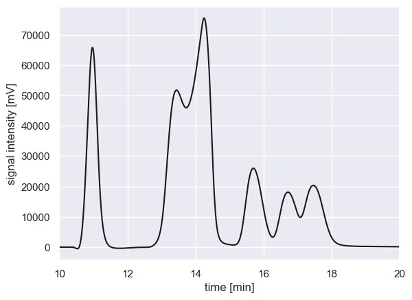
As an example, we can load a real chromatogram of a minimal medium for bacterial growth which has a slew of compounds, some of which overlap.

import pandas as pd
import matplotlib.pyplot as plt
import seaborn as sns
sns.set()

# Load a sample chromatogram and show the trace, cropped between 10 and 20 minutes
df = pd.read_csv('data/sample_chromatogram.txt')
plt.plot(df['time_min'], df['intensity_mV'], 'k-')
plt.xlabel('time [min]')
plt.ylabel('signal intensity [mV]')
plt.xlim([10, 20])

(10.0, 20.0)

With this signal, the location of peaks (meaning, the index where a local maxima is detected) can be identified using scipy.signal.find_peaks, even with a very low prominence filter. TO allow prominence filters to be comparable between chromatograms, we normalize the chromatogram first between 0 and 1.

import scipy.signal

# Create a normalized signal
signal_norm = (df['intensity_mV'] - df['intensity_mV'].min()) / (df['intensity_mV'].max() - df['intensity_mV'].min())

# Find peaks with a low prominence filter of 0.01
peak_locations, _ = scipy.signal.find_peaks(signal_norm, prominence=0.01)

# Plot the  original trace and overlay vertical lines with location of peaks
plt.plot(df['time_min'], signal_norm, 'k-', label='normalized chromatogram')
plt.vlines(df['time_min'].values[peak_locations], 0, 1, linestyle='--',
           color='dodgerblue', label='peak location')
plt.xlabel('time [min]')
plt.ylabel('normalized signal intensity')
plt.xlim([10, 20])
plt.title('prominence filter = 0.01')
plt.legend()

<matplotlib.legend.Legend at 0x16b293640>

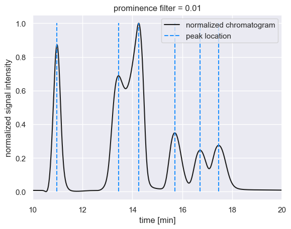
These maxima have prominence values greater than or equal to 0.01, meaning that maxima with prominences as low as 0.01 units above the local background are considered to be bonafide peaks. Increasing the prominence filter begins to remove peaks we would otherwise care about.

# Plot the  original trace and overlay vertical lines with location of peaks
fig, ax = plt.subplots(4, 1, figsize=(6, 8), sharex=True)
for a in ax:
    a.plot(df['time_min'], signal_norm, 'k-')
    a.set_ylabel('normalized\nsignal intensity')

# Plot for a few prominecne values
for i, p in enumerate([0.01, 0.1, 0.3, 0.5]):
    peak_locations, _ = scipy.signal.find_peaks(signal_norm, prominence=p)
    ax[i].vlines(df['time_min'].values[peak_locations], 0, 1, linestyle='--', color='dodgerblue')
    ax[i].set_title(f'prominence filter = {p}')

# Add necessary labels
ax[3].set_xlabel('time [min]')
ax[2].set_xlim([10, 20])
plt.tight_layout()

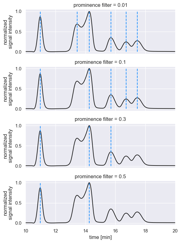
The choice of a prominence filter is going to be dependent on the size of peaks that you care to resolve in your chromatogram, their degree of overlap, and how noisy your signal is. The prominence filter can be passed as a keyword argument in the fit_peaks method of a Chromatogram. For example, passing a restrictive prominence filter of 0.1 can be done as follows:

from hplc.quant import Chromatogram

# Load the signal trace as a Chromatogram object and crop between 10 and 20 min.
chrom = Chromatogram(df, cols={'time':'time_min', 'signal':'intensity_mV'},
                     time_window=[10, 20])

# Pass a prominence filter, fit the peaks, and show the result
peaks = chrom.fit_peaks(prominence=0.1)
chrom.show()

Performing baseline correction: 100%|██████████| 299/299 [00:00<00:00, 3788.10it/s]
Deconvolving mixture: 100%|██████████| 2/2 [00:02<00:00,  1.03s/it]

[<Figure size 640x480 with 1 Axes>,
 <Axes: xlabel='time_min', ylabel='intensity_mV (baseline corrected)'>]

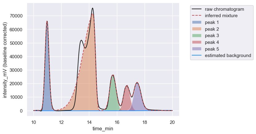
Note that even though the small peak at ≈ 13 minutes was not detected by the prominence filter, hplc-py still attempted to fit its signal as if it was part of the peak with a maximum at ≈ 14.2 min. This because the small peak was considered part of the same window of the major peak, as we will explore next.

Clipping the signal into peak windows

Once peak maxima are identified, hplc-py slices the chromatograms into windows–regions of the chromatogram where peaks are overlapping or nearly overlapping. This is achieved by measuring the widths of each peak at the lowest contour line. Peaks which have overlapping contour lines are considered to be close enough that their signals may be influencing one another. This is achieved under the hood in a method _assign_peak_windows of a Chromatogram which is called as part of fit_peaks.

# Fit the peaks using a permissive prominence filter
window_df = chrom._assign_windows(prominence=0.01)

# Plot each window
for g, d in window_df.groupby('window_id'):
    plt.plot(d['time_min'], d['intensity_mV'], '-', lw=3, label=f' window: {g}')
plt.xlabel('time [min]')
plt.ylabel('signal [mV]')

plt.legend()

<matplotlib.legend.Legend at 0x16b494790>

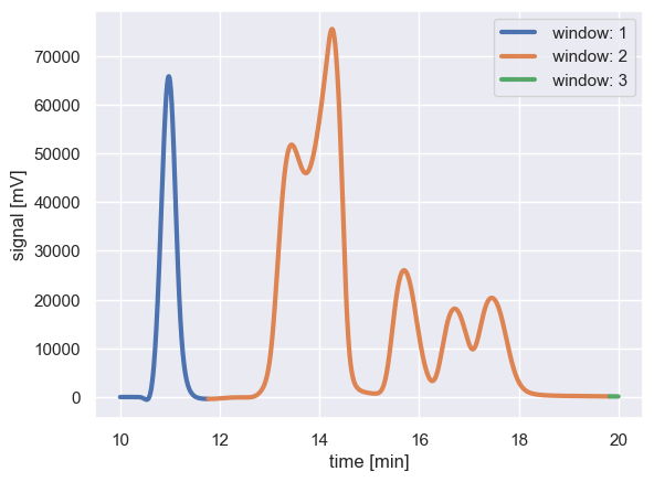
Peaks within each colored region are considered to be interacting signals, and are fit together as one unit. In the above example, the peak at ≈ 11 min (in window 1) is considered to be isolated from the peaks at ≈ 13 min onward.

The extent of each peak window can be controlled by a buffer parameter passed to fit_peaks and _assign_windows. This, given in units of time points, extends each peak window on to account for nearby baseline signal. The above windows can be expanded by increasing this parameter, which has a default value of 0.

# Increase the buffer and plot the change in the peak window.
buffer = 75
window_df = chrom._assign_windows(prominence=0.01, buffer=buffer)

# Plot each window
for g, d in window_df.groupby('window_id'):
    plt.plot(d['time_min'], d['intensity_mV'], '-', lw=3, label=f' window: {g}')
plt.xlabel('time [min]')
plt.ylabel('signal [mV]')
plt.title(f'buffer size = {buffer}')
plt.legend()

<matplotlib.legend.Legend at 0x16b65d240>

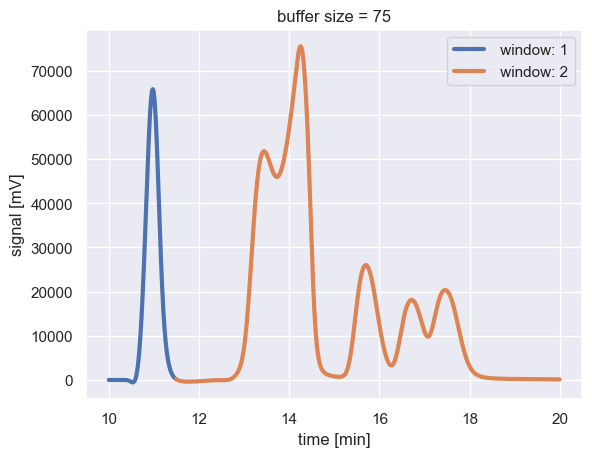
Note that increasing the buffer size expanded the extent of the orange window by half a minute or so.

Once the chromatogram is clipped into peak windows, each window is passed to an inference stage where the peak mixture is inferred.

---

© Griffin Chure, 2024. This notebook and the code within are released under a Creative-Commons CC-BY 4.0 and GPLv3 license, respectively.