7 Fitting and the importance of Regression
Once data have been visualized and explored, the next step is to move beyond descriptive plots and toward quantitative descriptions of patterns and relationships. This commonly involves fitting a function to data in order to summarize trends, extract parameters, or enable comparisons across conditions.
At a basic level, fitting refers to the process of relating observed data to a mathematical function. However, it is important to realize that the term fitting is often used very broadly, a bit of a semantic mess. An important conceptual distinction is between interpolation, smoothing, and regression.
7.1 Interpolation
Interpolation aims to describe the data between observed points by constructing a curve that passes exactly through all measurements. In this setting, the data points themselves are treated as if they were exact. Interpolation is therefore purely descriptive and is often the default behavior in plotting packages like Python’s Matplotlib, where lines are drawn directly between data points to guide the eye.
While this can be visually appealing, it is rarely appropriate for biological data, which are inherently noisy. Interpolated curves can give a misleading impression of precision and may obscure the underlying variability in the measurements.
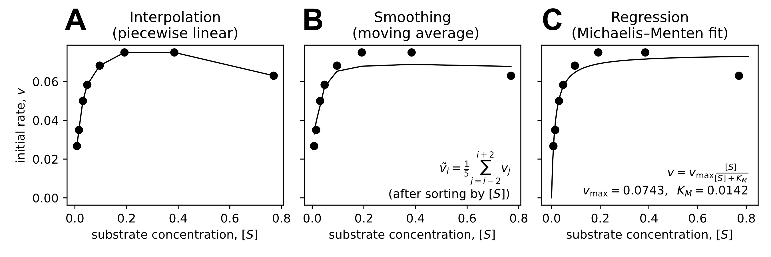
As an example, Fig. 7.1A shows the interpolation to the original enzyme activity data from Michaelis and Menten. Drawing an interpolated curve through all data points suggests a well-defined relationship between substrate concentration and activity, but such a curve does not provide quantitative biological information, such as the Michaelis–Menten constant \(K_M\).
7.2 Smoothing
Smoothing is also descriptive, but unlike interpolation it deliberately allows deviations from individual data points in order to reduce the influence of noise and reveal broader trends. Examples include moving averages or locally weighted smoothing methods.
In biological contexts, smoothing can be useful for visualizing overall behavior in noisy time-series data, such as growth curves, fluorescence traces, or sensor measurements. It can also be useful for identifying boundaries in image data. However, smoothing introduces subjective choices (such as window size or kernel shape) that affect the resulting curve. And like interpolation, smoothing does not by itself provide a framework for parameter estimation or evaluating a specific model or relationship between data.
An example of smoothing applied to the original Michaelis–Menten data and using moving averages is shown in Fig. 7.1B.
7.3 Regression
Regression, in contrast, treats observed data as noisy realizations of an underlying relationship and assumes a specific functional form. It explicitly acknowledges variability and seeks to estimate the parameters of that function such that it best describes the data.
Returning to the Michaelis–Menten example, a regression approach allows us to estimate the parameters \(K_M\) and \(v_{\max}\) of the Michaelis–Menten relation \[v = v_{\max}\frac{S}{S + K_M},\] where \(v_{\max}\) denotes the maximal reaction rate and \(K_M\) the substrate concentration at half-maximal rate, biologically important quantities. For the original data from Michaelis and Menten, the regression to this function is shown in Fig. 7.1C.
7.4 The importance of regression
Notably, regression provides not only point estimates of biologically meaningful parameters. Systematic regression also allows comparison across conditions and quantification of trends. For example, regression is the starting point to rigorously answer whether one enzyme operates faster than another, or whether cell growth across two conditions differ systematically. Regression is also crucial in many experimental workflows. Calibration curves, background correction, and baseline subtraction all rely on fitting specific functions to data in order to convert raw measurements into biologically meaningful quantities. In summary, regression is essential for quantitative biological data analysis. We next introduce the basic ideas underlying regression algorithms.
The term originates from the historical concept of “regression to the mean,” but in modern data analysis it refers more generally to modeling relationships between variables in the presence of noise, as introduced above.