20 The Dynamical Relation Between mRNA and Proteins
Optional topic. Weeks 8 and 9 (dynamical systems and nonlinear dynamics) are an optional part of the course.
To demonstrate the power of differential equations, we now apply this framework to one of the most fundamental biological processes: the dynamical relationship between gene expression, mRNA, and protein levels. Understanding this relationship better is essential to interpretate transcriptomic and proteomic data.
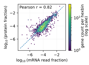
As a concrete example, consider the previously discussed steady growth of E. coli on glucose. Across genes and expression levels, protein abundances are strongly tied to mRNA abundance, as illustrated by the relationship between relative transcript and protein fractions derived from omics data (Fig. 20.1). Importantly, the shown correlation represents only a static snapshot of a highly dynamic process. To understand how such correlation patterns arise and to move toward a dynamical description, we turn to the central dogma of molecular biology: \[\text{DNA} \rightarrow \text{RNA} \rightarrow \text{protein}.\]
Rather than viewing this as a simple flow chart, we now setup a dynamical model of the central dogma. Consider a specific gene and let \(m(t)\) denote the number of mRNA molecules and \(p(t)\) the number of protein molecules in a cell for that specific gene. The fundamental processes of transcription, translation, and degradation can then be described by two coupled differential equations.
We begin with mRNA dynamics. The change in mRNA abundance due to transcription and degradation is given by \[\frac{dm}{dt} = G\kappa - \delta_{\mathrm{mRNA}}\, m.\]
Here, \(G\) denotes the copy number of the gene on the chromosome, and \(\kappa\) is an effective transcription rate (mRNA per unit time) describing how rapidly RNA polymerases produce transcripts from this gene. The parameter \(\delta_{\mathrm{mRNA}}\) is the mRNA degradation rate. The degradation term is proportional to \(m\) because each individual mRNA molecule has a certain probability per unit time to be degraded. When more mRNA molecules are present, more degradation events occur per unit time.
We can similarly describe the dynamics of protein molecules \(p\): \[\frac{dp}{dt} = \gamma\, m - (\delta_p + \lambda)\, p.\]
Here, \(\gamma\) is the translation rate (proteins produced per mRNA per unit time), and \(\delta_p\) is the protein degradation rate. In growing cell cultures, protein numbers are also reduced by cell division. This process, known as dilution, scales with the growth rate \(\lambda\) and is often more important than active degradation in fast-growing cells.
Together, these differential equations provide a simple model for the coupled dynamics of transcription and protein synthesis. Notice their hierarchical structure: protein dynamics depend on mRNA, while mRNA dynamics are independent of protein. This reflects the directionality of the central dogma. When we later consider gene regulation, this strict one-way dependence will be relaxed, giving rise to feedback loops and more complex dynamical behavior.
20.1 Estimating Gene Expression Parameters in Cells
As with every differential equation model, connecting the central-dogma model to real biology requires specifying realistic values for all model parameters. Importantly, these parameters are not abstract fitting constants, but correspond to measurable biological quantities, made possible by more than a century of methodological advances and elegant experiments in molecular biology. In the following we focus on E. coli numbers and specifically the gene lacZ, providing short order of magnitude estimations for each parameter.
Transcription rate \(\kappa\).
In E. coli, RNA polymerases operate with an elongation speed of approximately \(60~\mathrm{nt/s}\) when synthesizing mRNA. The time required to complete a transcript therefore depends on gene length. For LacZ, for example, transcription takes about \[\tau_{\mathrm{trs}} \approx 0.85~\mathrm{min}.\] The maximal transcription rate is given by the inverse of this, \[\kappa_{\max} \approx \frac{1}{\tau_{\mathrm{trs}}} \approx 70~\mathrm{h^{-1}}.\]
In real cells, however, transcription rates are typically much lower. Initiation is limited by promoter strength and by the availability of RNA polymerase. As a very rough argument, consider that about \(1000\) RNA polymerases are shared to transcribe roughly \(4000\) genes. The effective transcription capacity per gene is therefore expected to be several-fold lower than \(\kappa_{\max}\). We therefore use in our estimation and effective value \[\kappa \sim 17~\mathrm{h^{-1}}\] as an order-of-magnitude estimate.
Gene copy number \(G\).
The factor \(G\) accounts for gene copy number, which can exceed one in fast-growing cells due to multi-fork replication (cells maintain several copies of the chromosome which they replicate in parallel to make sure chromosome replication does not become a major bottleneck in growth). Here, we consider a single-copy situation only with \(G \approx 1\).
mRNA degradation rate \(\delta_{\mathrm{mRNA}}\).
Radiolabeling and transcriptional shutoff experiments have reported mRNA half-lives in E. coli of approximately \[\tau_{1/2} \approx 5~\mathrm{min}.\] For order-of-magnitude estimates, the degradation rate follows as a reciprocal of this timescale, \[\delta_{\mathrm{mRNA}} \approx \frac{1}{\tau_{1/2}} \approx 12~\mathrm{h^{-1}}.\]
Translation rate \(\gamma\).
Ribosomes synthesize proteins at a rate of about \(20~\mathrm{AA/s}\). For LacZ, this corresponds to a time to synthesize the protein of roughly \[\tau_{\mathrm{tsl}} \approx 1.3~\mathrm{min}.\] The throughput of a single translating ribosome is therefore approximately \[\gamma \approx \frac{1}{\tau_{\mathrm{tsl}}} \approx 46~\mathrm{h^{-1}}.\]
Protein degradation rate \(\delta_p\).
Most proteins in steadily growing E. coli are relatively stable and have long half-lives, often on the order of \[\tau_{1/2,\mathrm{prot}} \approx 30~\mathrm{h}\] or longer. The corresponding degradation rate is therefore small, \[\delta_p \approx \frac{1}{\tau_{1/2,\mathrm{prot}}} \approx 0.03~\mathrm{h^{-1}}.\]
Growth rate \(\lambda\) (dilution).
For growth on glucose, a typical doubling time is \[T_d \approx 1~\mathrm{h}.\] This corresponds to a growth rate of order \[\lambda \approx \frac{1}{T_d} \approx 0.45~\mathrm{h^{-1}}.\]
In this regime, dilution by growth dominates protein removal, \[\lambda \gg \delta_p,\] so active protein degradation can often be neglected to first order.
| Parameter | Meaning | Estimate (\(\mathrm{h^{-1}}\)) | How estimated |
|---|---|---|---|
| \(\lambda\) | growth rate (dilution) | \(\sim 0.5\) | doubling time \(T_d\approx 1~\mathrm{h}\) |
| \(\delta_{\mathrm{mRNA}}\) | mRNA degradation | \(\sim 12\) | mRNA half-life \(t_{1/2}\approx 5~\mathrm{min}\) |
| \(\delta_p\) | protein degradation | \(\sim 0.03\) | protein half-life \(t_{1/2}\approx 30~\mathrm{h}\) |
| \(\gamma\) | translation (effective) | \(\sim 46\) | LacZ synthesis time \(t_{\mathrm{synth}}\approx 1.3~\mathrm{min}\) |
| \(\kappa_{\max}\) | max transcription throughput | \(\sim 70\) | RNAP speed \(\sim 60~\mathrm{nt/s}\), LacZ length |
| \(\kappa\) | effective transcription rate | \(\sim 17\) | RNAP limitation + initiation efficiency |
| \(G\) | gene copy number | \(1\) or larger | replication state / locus position |
20.2 Steady-State Expression Levels
With all parameters specified, we can now analyze how transcription, translation, and degradation determine protein abundance. We begin by considering steady-state conditions, in which production and removal are balanced for both mRNA and protein.
Mathematically, steady state corresponds to \(dm/dt = dp/dt = 0\). Setting \(dm/dt = 0\) gives \[m^* = \frac{G\kappa}{\delta_{\mathrm{mRNA}}},\] and setting \(dp/dt = 0\) with \(m = m^*\) yields \[p^* = \frac{\gamma\, m^*}{\delta_p + \lambda} = \frac{\gamma\, G\kappa}{\delta_{\mathrm{mRNA}}(\delta_p + \lambda)}.\]
This expression has a clear biological interpretation: under steady-state conditions, protein abundance is determined by total synthesis divided by total removal. Transcription, translation, degradation, and growth together set the mRNA and protein levels through these balances.
Using the order-of-magnitude parameter values estimated above, we estimate for a steady state \[m^* \sim 1 \quad \text{and} \quad p^* \sim 10^2,\] Roughly one mRNA molecule and on the order of one hundred protein molecules per gene are present in a cell. While the exact values vary substantially across genes and conditions, the order of magnitudes have been confirmed in cells and highlight an important general feature of gene expression: mRNA copy numbers are often very small, whereas protein copy numbers are typically much larger.
This separation of scales has important consequences. Low mRNA copy numbers make transcription intrinsically noisy, while higher protein copy numbers provide partial buffering and stability at the protein level. We will come back to this point when analyzing stochastic processes.
Notably, for the steady growth of E. coli on glucose discussed earlier, many parameters in this expression, including \(\gamma\), \(\delta_{\mathrm{mRNA}}\), \(\delta_p\), and \(\lambda\), are approximately constant and shared across genes. In this regime, most gene-to-gene variation in protein abundance arises primarily from differences in transcriptional activity, encoded in \(G\kappa\). As a result, the model predicts the near-proportional relationship between mRNA and protein levels observed in the data (Fig. 20.1, blue line). Deviations from this simple relationship indicate additional layers of regulation, such as gene-specific translation efficiencies, differential protein stability, or post-transcriptional control.
Taken together, these steady-state relations define an important baseline or null model for gene expression. When most kinetic parameters are shared across genes, variation in protein abundance is dominated by transcriptional activity, and mRNA and protein levels are expected to scale proportionally. This provides a simple reference point against which more complex regulatory effects can be identified.
20.3 Response Dynamics and Timescales
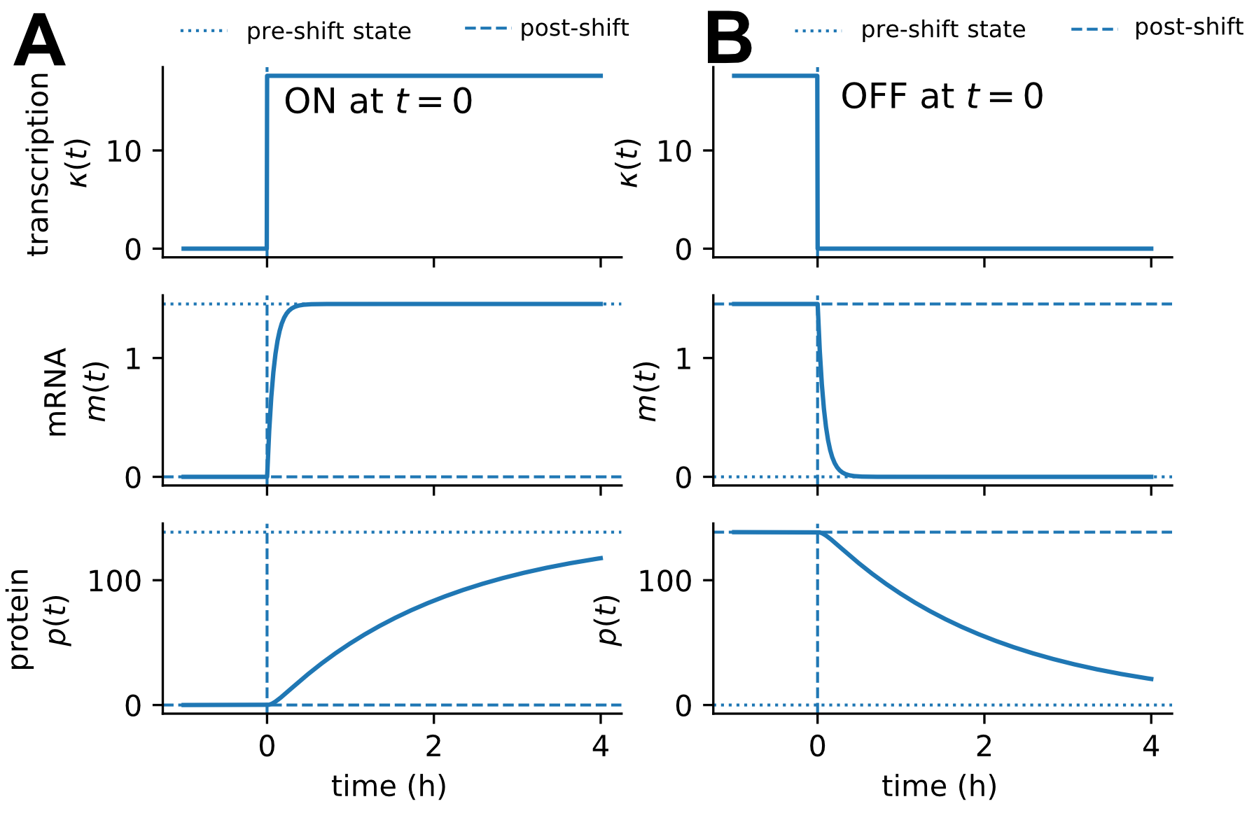
The same framework also naturally extends beyond steady-state conditions to describe how expression levels change in time. We here use the model to illustrate how mRNA and protein levels respond when gene expression is switched abruptly on or off at time \(t=0\). A numerical simulation of such a scenario is shown in Fig. 20.2.
When transcription is activated, mRNA levels rise rapidly, followed more slowly by protein accumulation. Conversely, when transcription is shut off, mRNA decays quickly, while protein levels decline more gradually. These distinct responses reflect the different characteristic timescales of RNA and protein turnover. In many cells, mRNA half-lives are typically on the order of minutes or tens of minutes, whereas many proteins are removed primarily by dilution through growth. As a result, transcript levels track regulatory changes much more rapidly than protein levels, which integrate cellular history over longer times.
These differential timescales are not merely a modeling detail, they impose fundamental physiological constraints. Because proteins accumulate and decay slowly, cells cannot instantaneously reconfigure their proteome in response to environmental change. This limitation helps explain phenomena such as apparent overcapacity in certain protein types and anticipatory synthesis of proteins before they are strictly required. In this way, simple dynamical considerations already provide insight into broader bacterial growth strategies and resource allocation principles.
So far, we have considered deterministic and linear models of gene expression. In reality, regulatory feedback and molecular noise introduce nonlinearity and variability, leading to richer dynamical behaviors. These effects will be explored in the following lectures.