8 Linear regression
While biological systems are generally nonlinear, linear regression is the most fundamental form of regression and underlies many methods in data analysis, including many machine-learning approaches. Linear regression appears frequently in biological data analysis as well, for example in calibration curves, growth-rate estimation, and dimensionality reduction of omics data.
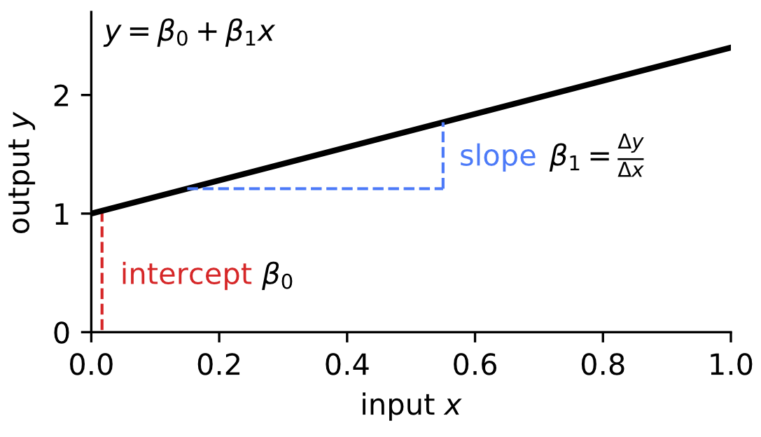
Mathematically, linearity means that changes in input lead to proportional changes in output and that the effects of multiple inputs add together. In the simplest case (1D), the relationship between an input variable \(x\) and an output variable \(y\) is described by a line, \[y = \beta_0 + \beta_1 x,\] where \(\beta_0\) is the intercept and \(\beta_1\) is the slope (Fig. 8.1).
Throughout this section, we refer to variables such as \(x\) as predictors (or input variables) and to \(y\) as the response (or output variable). Predictors are quantities used to explain or predict variation in the response. In biological contexts, predictors often represent experimentally controlled or observed inputs (e.g. substrate concentration, time, or treatment), while the response represents the measured outcome (e.g. reaction rate, growth rate, or expression level).
8.1 Linear regression as an optimization problem
Assume we have a set of \(n\) data points, \(\{(x_i, y_i)\}\), with \(i\) varying between \(1\) and \(n\). Linear regression asks the following question: how do we choose the parameters \(\beta_0\) and \(\beta_1\) such that the line those parameters define best describes the data?
Regression turns this question into an optimization problem by introducing a loss function that quantifies the mismatch between the line predictions and the observed data. A commonly used choice is the ordinary least squares (OLS) loss, defined as \[L(\beta_0, \beta_1) = \sum_{i=1}^n \left(y_i - \beta_0 - \beta_1 x_i\right)^2.\]
The goal of linear regression is to find the values of \(\hat{\beta}_0\) and \(\hat{\beta}_1\) that minimize this loss function. Intuitively, this corresponds to finding the line that minimizes the total squared vertical distance (\(\delta y\)) between the data points and the line.
Notably, this optimization problem can be solved analytically with basic concepts from differential calculus. We illustrate this in the following box for the intercept \(\hat{\beta}_0\). The slope \(\hat{\beta}_1\) can be derived similarly. For the following sections, it is most important to realize that the regression procedure has a well-defined mathematical foundation. Furthermore, because analytical solutions to the optimization problem exist, linear regression can be readily applied to data.
To find the values \(\beta_0\) and \(\beta_1\) where the loss function is minimal, we need to identify the stationary point of \(L\) where the partial derivatives with respect to \(\beta_0\) and \(\beta_1\) vanish.
Here, we focus on \(\beta_0\).
We require \[\frac{\partial L}{\partial \beta_0}\bigg|_{\hat{\beta}_0} = 0.\]
Computing the derivative, \[\begin{align} \frac{\partial L}{\partial \beta_0} &= \frac{\partial}{\partial \beta_0} \sum_{i=1}^n (y_i - \beta_0 - \beta_1 x_i)^2 \\ &= -2 \sum_{i=1}^n (y_i - \beta_0 - \beta_1 x_i). \end{align}\]
Setting this expression to zero at \(\hat{\beta}_0\) yields \[\hat{\beta}_0 = \bar{y} - \beta_1 \bar{x},\] where \(\bar{x}\) and \(\bar{y}\) denote the sample means of \(x\) and \(y\). Thus, we arrive at an equation stating how the optimal intercept depends on the provided data provided we know \(\beta_1\). With a similar approach for \(\beta_1\) we get a full solution stating how both, optimal intercept and slope, depend on data points alone.
Linear regression is one of the few regression types in which closed-form analytical solutions exist. This property underlies its importance in statistics and data analysis.
8.2 Example: Michaelis–Menten data via a linearizing transformation
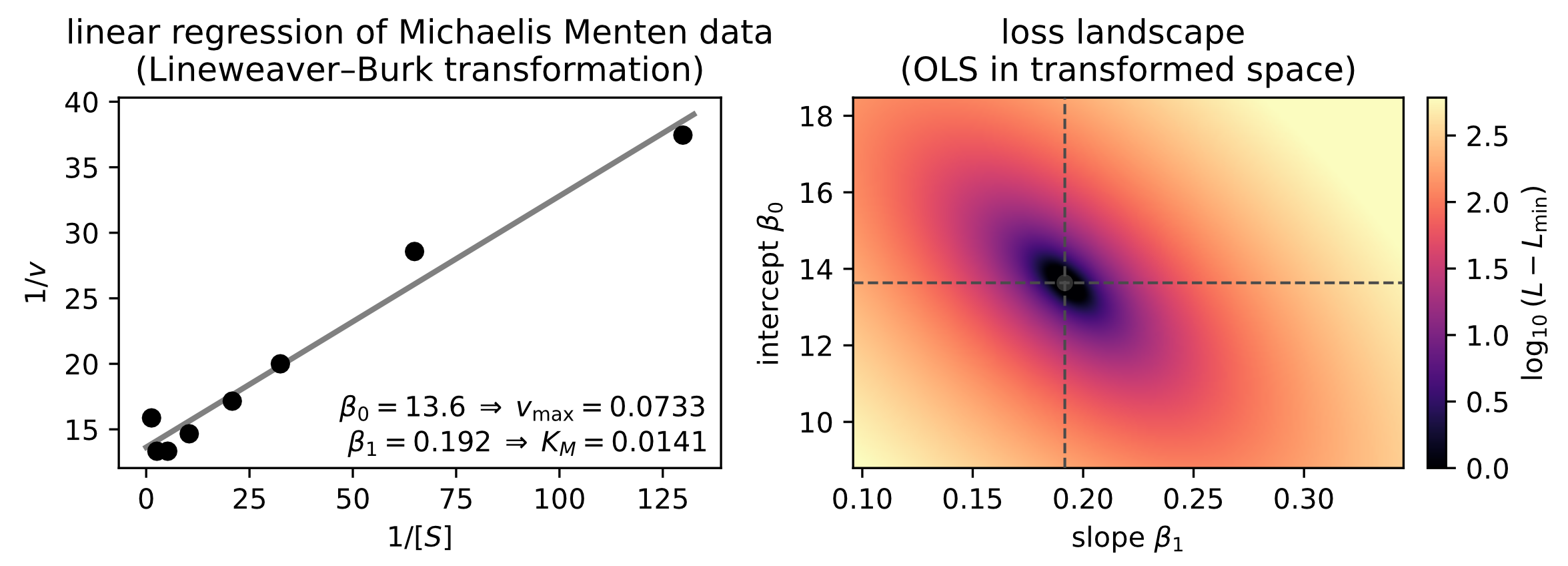
As a concrete biological example, we apply linear regression to the original enzyme kinetics data from Michaelis and Menten. As with many fundamental relations in biology, the relationship between substrate concentration and reaction rate is highly nonlinear. However, it can be transformed into a linear relationship that can be fit with a straight line. Figure 8.2A shows the resulting linear fit, the inferred slope and intercept parameters, and the resulting parameters \(K_m\) and \(v_{max}\) of the Michaelis–Menten relation. Figure 8.2B shows the loss function for different slope and intercept parameters, confirming the identification of both parameters where the loss function is lowest.
Notably, a closely related quantity is the Pearson correlation coefficient, which measures the strength of linear association between two variables. If both \(x\) and \(y\) are standardized to have mean zero and variance one, then the slope \(\hat{\beta}_1\) of the linear regression equals the Pearson correlation coefficient. Thus, correlation and linear regression capture closely related information, though they typically serve different analytical purposes.
To see this, let’s consider the OLS slope of a linear regression of \(Y\) on \(X\). \[\begin{align*} \hat{\beta}_1 &= \frac{\sum_i (x_i - \overline{x})(y_i - \overline{y} )}{\sum_i (x_i - \overline{x})^2}\\ &= \frac{\sum_i (x_i - \overline{x})(y_i - \overline{y} )}{\sqrt{\sum_i (x_i - \overline{x})^2} \sqrt{\sum_i (y_i - \overline{y})^2}} \cdot \frac{\sqrt{\sum_i (y_i - \overline{y})^2}}{\sqrt{\sum_i (x_i - \overline{x})^2}}\\ &= p_{xy} \cdot \frac{s_y}{s_x}, \\ \end{align*}\]
where \(p_{xy}\) is the Pearson correlation, and \(s_x\) and \(s_y\) are the standard deviation of \(x\) and \(y\) respectively. Therefore the slope can be rewritten as the Pearson correlation scaled by the standard deviation of the two variables.
8.3 Generalization to multiple predictors and multiple linear regression
The univariate linear regression discussed above, fitting a line to relate a single predictor variable to a response variable, is a special case of linear regression. Here, univariate refers to the fact that only one predictor is used. In practice, we often measure multiple predictor variables simultaneously and wish to relate them to a single response variable.
Linear regression naturally generalizes to this setting, commonly referred to as multiple linear regression, using vector and matrix notation.
Let \[\mathbf{y} \in \mathbb{R}^n\] denote the vector of observed responses, \[\mathbf{X} \in \mathbb{R}^{n \times p}\] the design matrix containing the predictor variables, and \[\boldsymbol{\beta} \in \mathbb{R}^p\] the vector of regression coefficients. Each row of \(\mathbf{X}\) corresponds to one observation, and each column corresponds to one predictor.
The linear regression model can then be written compactly as \[\mathbf{y} = \mathbf{X}\boldsymbol{\beta} + \boldsymbol{\varepsilon},\] where \(\boldsymbol{\varepsilon}\) is a vector of residual errors capturing variability not explained by the linear relationship.
Despite involving multiple predictors, this model remains linear in the parameters \(\boldsymbol{\beta}\), which is the defining feature of linear regression. Univariate linear regression corresponds to the special case \(p=1\).
As in the univariate case, regression proceeds by minimizing the sum of squared residuals. The difference is that the prediction now combines contributions from multiple predictors: \[L(\boldsymbol{\beta}) = \|\mathbf{y} - \mathbf{X}\boldsymbol{\beta}\|^2.\]
Provided that the number of observations exceeds the number of parameters and that the columns of \(\mathbf{X}\) are not linearly dependent, this optimization problem admits an analytical solution, \[\hat{\boldsymbol{\beta}} = (\mathbf{X}^\top \mathbf{X})^{-1}\mathbf{X}^\top \mathbf{y}.\]
This expression highlights why linear algebra is central to linear regression. For high-dimensional biological datasets, such as omics data, advanced computational linear algebra methods are essential. In practice, tailored numerical algorithms are used rather than explicitly computing matrix inverses. These algorithms can be conveniently applied using different analysis packages, often designed for specific biological data types. We will return to these methods when discussing omics data analysis later in the course.
Linear regression is one of the few regression settings in which closed-form analytical solutions exist.
This makes it computationally efficient and conceptually transparent. However, it is good to know that the ordinary least squares (OLS) loss used here is only one specific choice of loss function. Other loss functions are also used, for example to reduce sensitivity to outliers or to emphasize different aspects of the data. Furthermore, even for linear regression, practical implementations often rely on numerical linear algebra methods, especially for large or high-dimensional datasets.