11 Sampling variability and the standard error of the mean
The law of large numbers states that sample averages converge toward true underlying values as more and more samples are taken. In practice, however, we always work with a finite number of samples. As a result, even when the law of large numbers applies, sample means retain residual variability due to finite sampling.
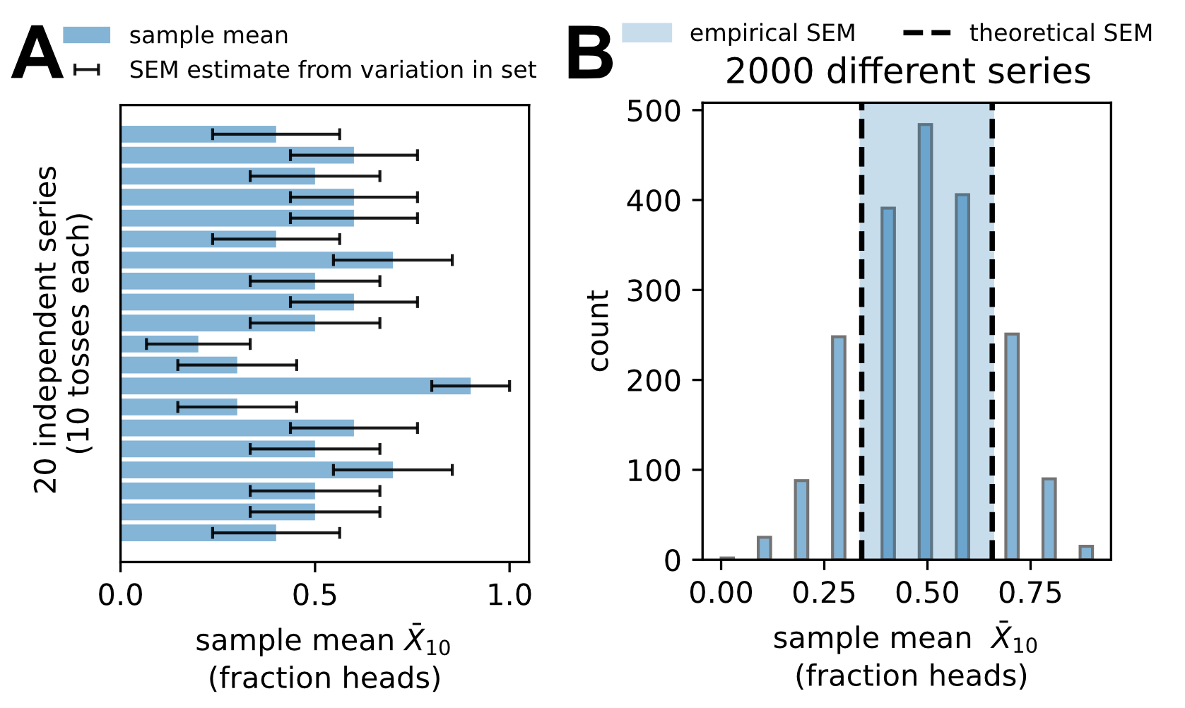
For example, consider again the coin-toss experiment. If we analyze multiple independent series of coin tosses, each consisting of, for example, 10 tosses, we find that the sample mean differs from series to series (Fig. 11.1A).
To quantify this uncertainty in the mean, it is helpful to formalize the problem as bit more.
For each series of \(n\) coin tosses, we compute the sample mean \[\bar{X}_n = \frac{1}{n} \sum_{i=1}^{n} X_i,\] where the \(X_i\) are independent random variables drawn from the same underlying distribution.
Because the individual measurements (or tosses) \(X_i\) are random variables, the sample mean \(\bar{X}_n\) is itself a random variable. Its value fluctuates from one series of coin tosses to another. This variability of the sample mean across repeated experiments quantifies the uncertainty in our estimate of the true mean. The key question is therefore: how large are these fluctuations of \(\bar{X}_n\), and how do they depend on the number of samples n?
11.1 The standard error of the mean
To quantify the fluctuations of the sample mean \(\bar{X}_n\), and thus the uncertainty in our estimate of the true mean, we consider the standard deviation of the mean, also called the standard error of the mean (SEM).
The standard deviation and the related variance are fundamental characteristics of a random variable, describing the spread of values (see box).
The variance and standard deviation quantify the spread of a random variable around its mean.
The variance measures the average squared deviation from the mean, which ensures that positive and negative deviations do not cancel and that larger deviations are weighted more strongly. The standard deviation is the square root of the variance and has the same units as the original measurement, making it easier to interpret.
For a discrete random variable \(X\) with mean \(\mu\) and probabilities \(P(X=x)\), the variance is defined as \[\mathrm{Var}(X) = \sum_x (x - \mu)^2 \, P(X = x).\]
The standard deviation is \[\sigma = SD(X)=\sqrt{\mathrm{Var}(X)}.\]
Notably, the SEM (the standard deviation of the mean) follows a very simple relation: If individual measurements fluctuate around the true mean with a typical spread characterized by a standard deviation \(\sigma\), then the standard error of the mean is given by \[\mathrm{SEM} = \frac{\sigma}{\sqrt{n}}.\]
Importantly, this formula follows directly from basic probability considerations. We show the derivation in the following box.
The standard error of the mean is defined as the standard deviation of the sample mean \(\bar{X}\): \[\mathrm{SEM} \equiv \mathrm{SD}(\bar{X}) = \sqrt{\mathrm{Var}(\bar{X})}.\]
We start by computing the variance of the sample mean: \[\begin{align*} \mathrm{Var}(\bar{X}) &= \mathrm{Var}\!\left(\frac{1}{n}\sum_{i=1}^n X_i\right) \\[4pt] &= \left(\frac{1}{n}\right)^2 \mathrm{Var}\!\left(\sum_{i=1}^n X_i\right) \qquad \text{(scaling rule)} \\[4pt] &= \frac{1}{n^2}\sum_{i=1}^n \mathrm{Var}(X_i) \qquad \text{(additivity rule)} \\[4pt] &= \frac{1}{n^2}\sum_{i=1}^n \sigma^2 \qquad \text{(identical distributions)} \\[4pt] &= \frac{\sigma^2}{n}. \end{align*}\]
Taking the square root yields the standard deviation of the mean: \[\mathrm{SEM} = \sqrt{\mathrm{Var}(\bar{X})} = \frac{\sigma}{\sqrt{n}}.\]
Note that this derivation made use of two basic rules:
Scaling: \(\mathrm{Var}(aZ)=a^2\,\mathrm{Var}(Z)\)
Additivity: for independent variables, \(\mathrm{Var}\!\left(\sum Z_i\right)=\sum \mathrm{Var}(Z_i)\)
The simple SEM formula highlights two important points. First, the standard error of the mean decreases with the number of measurements (e.g. coin tosses), reflecting the increasing precision of the sample mean as sample size grows. Second, the magnitude of the uncertainty depends on the variability of the underlying distribution. Measurements drawn from a broader distribution lead to larger uncertainty in the estimated mean.
In practice, the standard deviation \(\sigma\) characterizing this underlying variability is usually unknown. Instead, it is estimated from the observed spread of the data. As a consequence, the SEM formula provides a simple and practical way to estimate uncertainty in the mean directly from experimental measurements.
To build intuition for this uncertainty under realistic conditions, consider again the coin-toss example. If we repeat the coin-toss experiment many times—each time computing the sample mean—the distribution of these means becomes smooth and stable (Fig. 11.1B). The width of this distribution reflects the uncertainty in the mean, indicated by the blue shaded region. This width is well captured by the SEM predicted by the formula above (dashed black lines).
In real experiments, we rarely perform thousands of independent replicates. Instead, we estimate the uncertainty of the mean using the sample standard deviation and the SEM formula. This estimated uncertainty is commonly visualized using error bars, as shown for each coin-toss series in Fig. 11.1A.
Let us further clarify at this point the relation of the SEM to confidence intervals and standard deviations.
First, confidence intervals: The standard error of the mean quantifies how much the sample mean is expected to fluctuate due to finite sampling. Confidence intervals build on this idea by converting the SEM into a range of plausible values for the true mean. See box.
Under common assumptions—independent measurements and sufficiently large sample size—the distribution of the sample mean is approximately normal. In this regime, uncertainty in the mean can be summarized by \[\bar{X} \pm z \times \mathrm{SEM},\] where \(z\) is a factor determined by the desired confidence level.
For a 95% confidence interval, \[\bar{X} \pm 1.96 \times \mathrm{SEM},\] reflecting the fact that approximately 95% of values drawn from a normal distribution lie within 1.96 standard deviations of the mean.
Importantly, a 95% confidence interval does not assign a probability to a specific interval containing the true mean. Instead, it means that if the experiment were repeated many times, 95% of the resulting confidence intervals would contain the true mean.
Confidence intervals therefore provide a practical and interpretable way to communicate uncertainty and to compare estimates across conditions.
Second, it is important to clearly distinguish between the standard deviation and the standard error of the mean. These are related but conceptually distinc quantities and in the literature error bars are used to describe one or the other. See box.
Standard deviation (SD) quantifies the variability of individual measurements. It describes how spread out the data are and reflects biological heterogeneity, technical noise, or both.
For measurements \(X_1,\dots,X_n\) with sample mean \(\bar{X}\), the sample standard deviation is \[s = \sqrt{\frac{1}{n-1}\sum_{i=1}^n (X_i-\bar{X})^2}.\]
Standard error of the mean (SEM) quantifies uncertainty in the estimated mean due to finite sampling. It describes how much the sample mean would vary if the experiment were repeated many times under identical conditions: \[\mathrm{SEM} = \frac{s}{\sqrt{n}}.\]
Key distinction:
SD answers: How variable are individual measurements?
SEM answers: How precisely has the mean been estimated?
Error bars may represent SD, SEM, confidence intervals, or other quantities. Figures therefore always need to state explicitly what error bars represent.
11.2 Why normal distributions appear so often
Before we move on to bootstrapping, an easily applicable method for estimating uncertainty in quantities beyond the mean, we briefly comment on the central limit theorem (CLT). Alongside the law of large numbers, the CLT can be seen as a second major theorem in statistics that greatly simplifies statistical reasoning.
The CLT states that, under fairly general conditions, the distribution of sample means approaches a normal distribution as the sample size increases, regardless of the shape of the underlying measurement distribution. For example, in the coin-toss simulations considered above, the resulting distribution of sample means follows the familiar bell-shaped form of the normal distribution (Fig. 11.1B).
The theorem explains why quantities such as the standard error of the mean and confidence intervals are often expressed using normal distributions.
More broadly, the CLT rationalizes why many classical statistical methods are built around normal distributions. Methods such as Student’s t-tests for example build on normal distributions to provide simple analytical formulas for uncertainty estimation and hypothesis testing.
Importantly, however, the CLT relies on stronger assumptions than the law of large numbers. Moreover, similar to the law of large numbers it is an asymptotic result: it describes behavior only in the limit of large sample sizes. In most biological experiments, sample sizes are small and normal approximations as well as the statistical methods that rely on them, can be inaccurate or misleading.
For this reason, we emphasize computational approaches in this class, such as bootstrapping and permutation tests. These rely less on distribution assumptions and instead build uncertainty estimates directly from data.
11.3 Maximum likelihood estimation: fitting probability distributions
So far, we have estimated the mean by averaging repeated measurements. More generally, however, we often want to estimate parameters of an explicit probabilistic model from data. That is, we want to fit a probability distribution to data. Maximum likelihood estimation(MLE) provides a unifying framework for doing exactly this.
11.3.1 The key idea
The key idea of MLE is simple: we choose parameters of the probabilistic model such that the observed data are as likely as possible under the assumed probability model.
Concretely, suppose we observe data points \(X_1,\dots,X_n\) that are modeled as independent realizations of a random variable with probability distribution \(p(x\mid\theta)\), where \(\theta\) denotes an unknown parameter (or set of parameters). The likelihood is defined as the probability of the observed data, viewed as a function of \(\theta\), \[\mathcal{L}(\theta) = \prod_{i=1}^n p(X_i \mid \theta).\]
The maximum likelihood estimate \(\hat{\theta}\) is the parameter value that maximizes this likelihood.
Given observed data \(X_1,\dots,X_n\) and a probabilistic model \(p(x\mid\theta)\), the maximum likelihood estimate \(\hat{\theta}\) is defined as \[\hat{\theta} = \arg\max_{\theta} \; \mathcal{L}(\theta), \qquad \mathcal{L}(\theta)=\prod_{i=1}^n p(X_i \mid \theta).\]
The likelihood is written as a product because the data points are assumed to be independent. Independence implies that the probability of observing all data is the product of the probabilities of the individual observations.
11.4 Example: coin tossing as maximum likelihood estimation
Consider again the coin-toss experiment. We model each toss as a Bernoulli random variable, \[X_i = \begin{cases} 1 & \text{heads},\\ 0 & \text{tails}, \end{cases}\] with unknown probability \(p\) of obtaining heads.
Under this model, the probability of observing a particular sequence \(X_1,\dots,X_n\) is \[\mathcal{L}(p) = \prod_{i=1}^n p^{X_i}(1-p)^{1-X_i}.\]
This expression is the likelihood of the parameter \(p\) given the observed data, that is, it quantifies how plausible different values of \(p\) are. Maximizing \(\mathcal{L}(p)\) with respect to \(p\) yields a remarkably simple result: \[\hat{p} = \bar{X}_n,\] the sample mean of the observed coin-toss outcomes.
Note: We include this derivation to show that the result can be obtained explicitly. You do not need to follow every algebraic step; the key point is that the sample mean emerges as the maximum likelihood estimate.
Consider \(n\) independent coin tosses with outcomes \[X_1, X_2, \dots, X_n \in \{0,1\},\] where \(X_i=1\) denotes heads and \(X_i=0\) tails. Assume each toss follows a Bernoulli distribution with unknown probability \(p\) of heads.
The likelihood of observing the data is \[\mathcal{L}(p) = \prod_{i=1}^n p^{X_i}(1-p)^{1-X_i} = p^{\sum_i X_i}(1-p)^{n-\sum_i X_i}.\]
Rather than maximizing \(\mathcal{L}(p)\) directly, we maximize the log-likelihood: \[\ell(p) = \log \mathcal{L}(p) = \left(\sum_i X_i\right)\log p + \left(n-\sum_i X_i\right)\log(1-p).\]
Taking the derivative with respect to \(p\) and setting it to zero yields \[\frac{d\ell}{dp} = \frac{\sum_i X_i}{p} - \frac{n-\sum_i X_i}{1-p} = 0.\]
Solving for \(p\) gives \[\hat p = \frac{1}{n}\sum_{i=1}^n X_i = \bar X_n.\]
Thus, the maximum likelihood estimate of the probability of heads is simply the sample mean of the observed outcomes.
11.4.1 Least squares as maximum likelihood estimation
The maximum likelihood framework also explains why least squares regression appears so ubiquitously in data analysis.
Assume we model measurements by a straight line with additive noise, \[y_i = \beta_0 + \beta_1 x_i + \varepsilon_i,\] where the noise terms \(\varepsilon_i\) are independent and normally distributed with mean zero and variance \(\sigma^2\).
Under this assumption, each observation \(y_i\) is itself normally distributed around the model prediction, \[p(y_i \mid \beta_0,\beta_1) = \frac{1}{\sqrt{2\pi\sigma^2}} \exp\!\left[ -\frac{\bigl(y_i-(\beta_0+\beta_1 x_i)\bigr)^2}{2\sigma^2} \right].\]
Assuming independent measurements, the likelihood of the full dataset is the product of these Gaussian probabilities, \[\mathcal{L}(\beta_0,\beta_1) = \prod_{i=1}^n \frac{1}{\sqrt{2\pi\sigma^2}} \exp\!\left[ -\frac{\bigl(y_i-(\beta_0+\beta_1 x_i)\bigr)^2}{2\sigma^2} \right].\]
Maximizing this likelihood is equivalent to maximizing its logarithm. Notably, as we discuss further in an optional problem set, this is equivalent to minimizing the sum of squared residuals.
This is why ordinary least squares is typically used as the loss function in regression: least squares regression is the maximum likelihood estimator for the parameters of a straight-line model \(\beta_0+\beta_1 x\) under the assumption of independent Gaussian measurement noise.
In the next section, we will introduce bootstrapping, a complementary approach that allows uncertainty estimation without relying on an explicit probabilistic model.