12 Bootstrapping
To quantify uncertainties, we have so far focused on the sample mean, with the standard error of the mean (SEM) quantifying the uncertainty of an average. The SEM is powerful and theoretically well grounded in the law of large numbers, which applies broadly in biological settings and well-designed experiments. However, what if we want to quantify uncertainty in quantities beyond the mean, such as regression parameters, medians, or nonlinear model fits, for which simple analytical error formulas often do not exist? And what if we want to understand not just the size of uncertainty, but the shape of the uncertainty distribution itself?
One convenient and increasingly used approach for estimating uncertainty in such cases is bootstrapping. Unlike many statistical methods, bootstrapping does not require assuming a specific functional form for the underlying distribution of the data. Instead, it asks a simple empirical question: how much variability is already present in the data we have measured?
12.1 Resampling with replacement generate virtual realizations
The core idea of bootstrapping is the systematic resampling of the observed dataset. In practice, we let the computer mimic repeated experiments by repeatedly drawing from the available data. To illustrate this idea, consider again the coin toss example. Suppose we perform a coin toss experiment with \(n = 10\) tosses and record the outcomes (Fig. 12.1A).
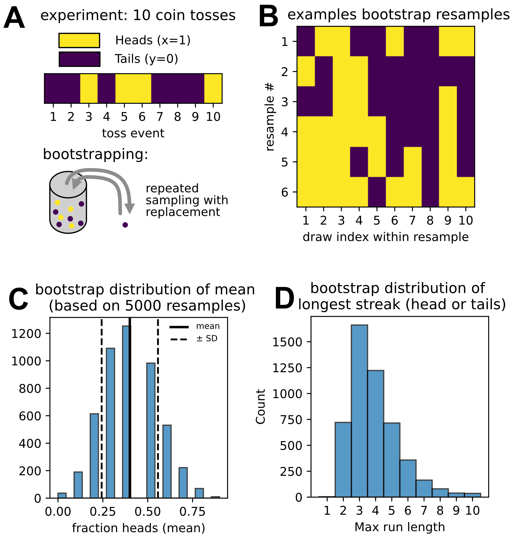
To simulate repeated experiments, we generate new datasets by sampling with replacement from these observed outcomes. Each resampled dataset has the same size as the original experiment but may contain repeated values and omit others (Fig. 12.1B). By repeating this resampling procedure many times, we generate many “virtual” realizations of the experiment.
12.2 Generating and analyzing bootstrap distribution for the quantity of interest
For each bootstrap sample, we then compute the statistic of interest, for example the mean fraction of heads. Repeating this procedure yields a distribution of bootstrap estimates for this quantity. This bootstrap distribution approximates the sampling distribution of the estimator: a wider distribution indicates greater sampling uncertainty, while a narrower distribution indicates higher precision. Fig. 12.1C shows an example for the mean of coin-tossing.
Bootstrapping is powerful because it approximates the full sampling distribution of a quantity of interest directly from the available data. This is particularly useful when we care about statistics beyond the mean, or when the shape of the uncertainty distribution itself is informative.
For example, once the bootstrap distribution has been obtained, it can be used to define confidence intervals. E.g. the 2.5th and 97.5th percentiles of the bootstrap mean distribution can be used to define a 95% bootstrap confidence interval. Another example for coin tossing is the statistics of longest streaks (either heads or tails only). The distribution resulting from bootstrapping is shown in Fig. 12.1D.
12.3 Practical implications
Because bootstrapping works for any statistic, not just means, it is particularly useful in biology, where data are often skewed and where meaningful summaries frequently go beyond averages. Quantities such as medians, regression slopes, and parameters of nonlinear models often lack simple analytical formulas for their uncertainty. Bootstrapping provides a general way to estimate uncertainty for these quantities directly from the data.
Furthermore, bootstrapping is straightforward to implement with modern computational tools. In the accompanying Jupyter notebook, we demonstrate how to implement bootstrapping in Python and apply it to examples where analytical uncertainty estimates are unavailable or inappropriate.
The bootstrap is a fairly new approach, introduced by Bradley Efron in 1979. While conceptually simple, its widespread use became practical only with fast computing. In the life sciences, bootstrapping has become increasingly common as datasets have grown larger and computational tools more accessible, enabling routine uncertainty estimation for complex statistics and models.
12.4 Bootstrapping to evaluate fitted parameters
So far, we have used bootstrapping to quantify uncertainty in simple summary statistics such as the mean. The same idea can be applied to evaluate uncertainty in fitted model parameters, even when analytical error estimates are unavailable.
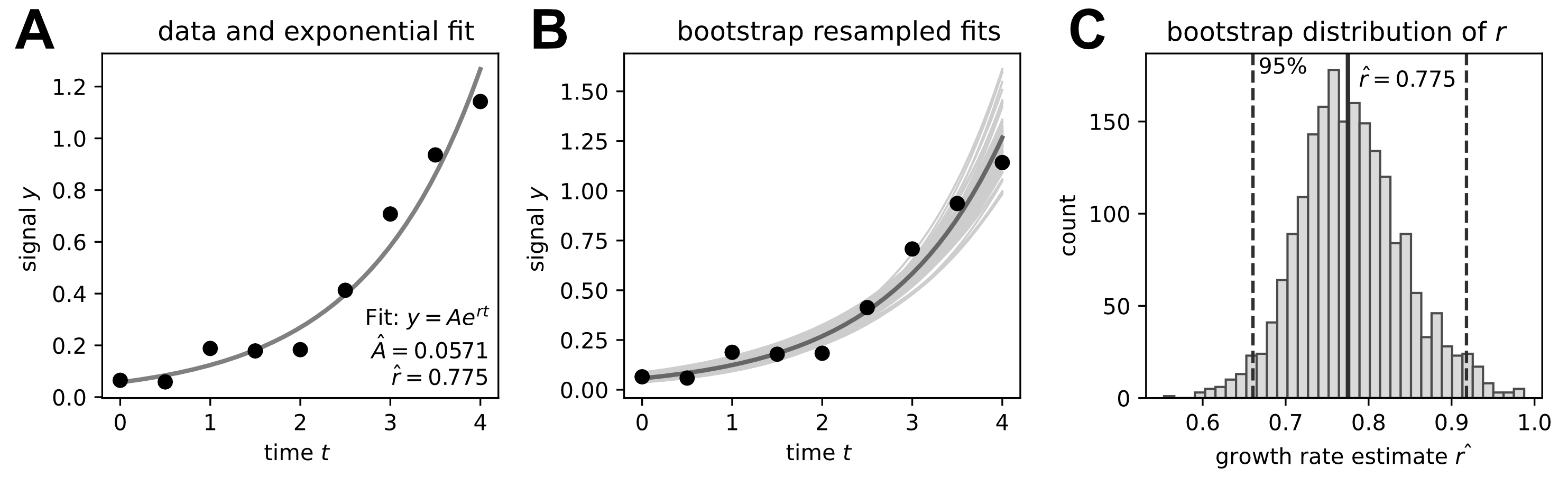
As a concrete example, consider fitting an exponential growth model \[N(t) = N_0\, e^{rt}\] to time-series data, where \(r\) denotes the growth rate. A standard regression fit yields a single best-fit estimate \(\hat r\) (Fig. 12.2A). However, due to measurement noise and finite sampling, this estimate is uncertain.
Bootstrapping provides a direct way to quantify this uncertainty. Starting from the observed growth curve, we generate many bootstrap datasets by resampling the measured data points \((t_i, N_i)\) with replacement (Fig. 12.2B). For each bootstrap dataset, we refit the exponential model and record the resulting growth rate. Repeating this procedure produces a bootstrap distribution of fitted growth rates (Fig. 12.2C).
The spread and shape of this bootstrap distribution reflect how sensitive the fitted parameter is to sampling variability in the data. A narrow distribution indicates that the growth rate is well constrained by the measurements, whereas a broad or skewed distribution signals substantial uncertainty or limited information content in the data.
Notably, this approach requires no analytical error formulas and applies equally to linear and nonlinear models. Bootstrapping is therefore a good general method for estimating uncertainty in fitted parameters.
12.5 Caveats and assumptions
While bootstrapping is very general, it does not eliminate the need for careful experimental design. Like analytical error estimates, bootstrap results rely on the assumption that the available data are representative of the underlying process. In particular, standard bootstrapping assumes statistically independent observations, analogously to the assumptions underlying the SEM introduced above (e.g., not time-correlated measurements or pseudo-replicates). Bootstrapping is therefore a powerful complement to analytical approaches, not a substitute for well-defined experiments or clearly identified biological replicates.