13 Hypothesis testing
In the previous section, we focused on estimating uncertainty: how precisely can we determine a quantity given a finite sample size and noisy data? In many biological settings, however, we want to go further and ask whether observed data are consistent with a proposed explenation or hypothesis. Hypothesis testing provides a statistical framework for addressing this question.
Crucially, hypothesis testing does not aim to directly assess whether a specific hypothesis is true, something that is generally very difficult, if not impossible, to establish conclusively. Instead, hypothesis testing evaluates whether the observed data are consistent with a baseline explanation, called the null hypothesis. If the data are highly inconsistent with the null hypothesis, this provides evidence against it and in favor of an alternative explanation.
13.1 Example: testing whether a coin is fair
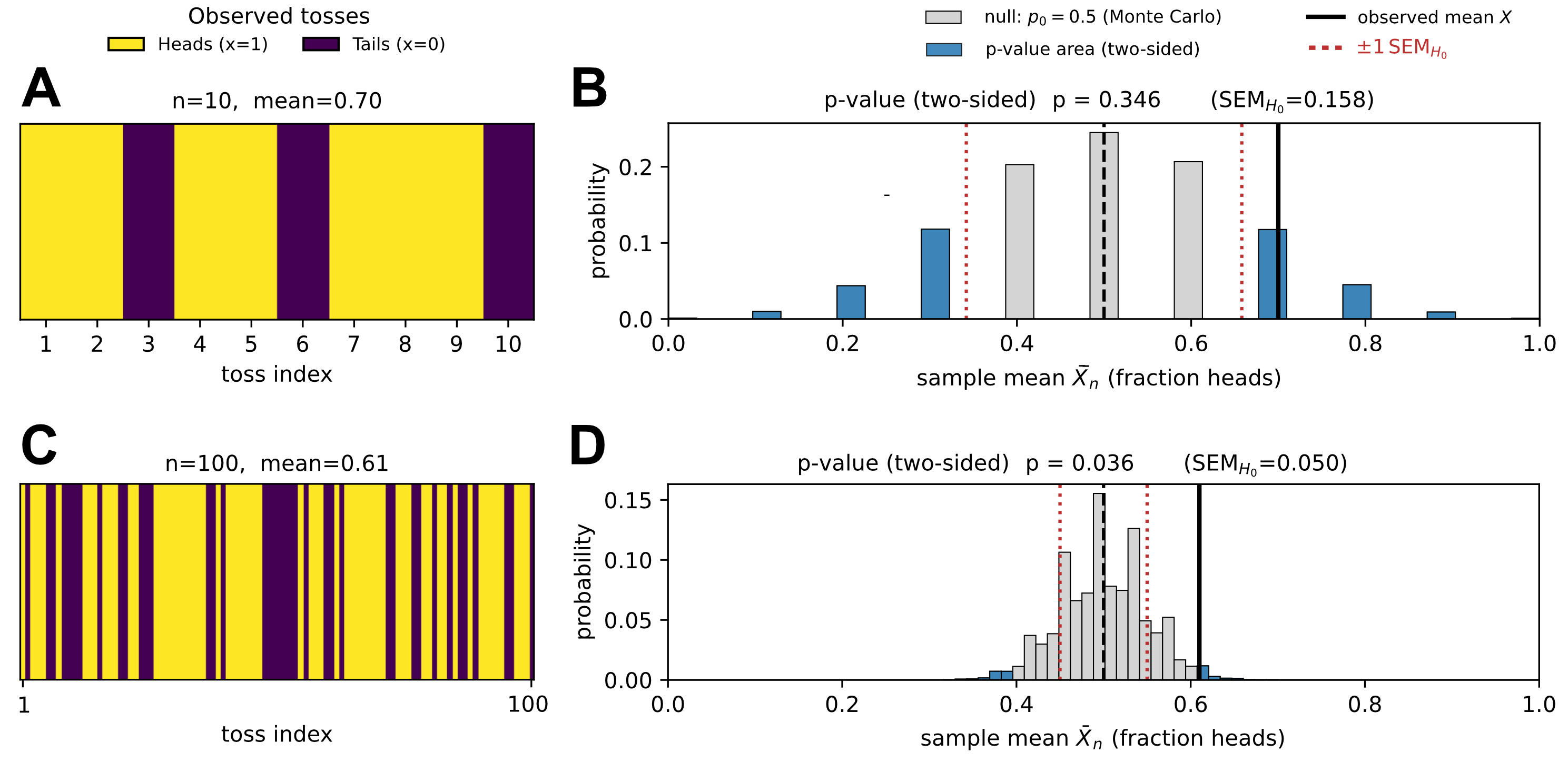
To introduce the core idea, consider again the coin-toss example introduced earlier. Suppose we toss a coin \(n = 10\) times and record heads as 1 and tails as 0. After performing the experiment, we compute the observed fraction of heads and obtain \(\bar X_n = 0.7\) as shown in Fig. 13.1A. As this fraction deviates substantially from 0.5, we may wonder whether the coin is not fair. That is, the coin is biased, not producing heads and tails with equal probability.
To evaluate this suspicion or hypothesis, we first formulate a null hypothesis: the coin is fair, with the probability of heads being \(p_{0} = 0.5\). Assuming this hypothesis is true, we can ask what outcomes we would expect from repeated coin tossing experiments with n=10 tosses each. Using a computer, we can simulate many independent series of 10 coin tosses under the assumption of a fair coin and record the resulting fractions of heads. The distribution of these simulated outcomes is shown in Fig. 13.1B.
We can now evaluate our observation \((\bar X_n = 0.7)\) relative to this reference distribution. Specifically, we ask: what fraction of simulated experiments would produce a result at least as extreme as the observed one? This fraction corresponds to the shaded region in Fig. 13.1B and is commonly called a p-value.
For 10 tosses, observing a fraction of heads larger as 0.7 (or 0.3 or smaller) is highly likely (about 37%) and compatible with the sampling variability expected under the assumption of a fair coin. That is, the p-value is about 0.35. Accordingly, with this experiment alone we cannot conclude that the coin is unfair. In other words, the observation do not provide strong evidence against the null hypothesis.
13.2 General steps of hypothesis testing
The coin-toss example already contains all essential ingredients of a hypothesis test. We now explicitly state the steps involved.
First, we need to formulate a null hypothesis. The null hypothesis represents a baseline explanation for the data. In the coin-toss example, the null hypothesis was that the coin is fair, meaning that the probability of heads is \(p_0 = 0.5\).
Second, we define a test statistic that summarizes the observed data in a single number. In the coin-toss experiment, a natural test statistic is the sample mean \[\bar X_n = \frac{1}{n} \sum_{i=1}^n X_i,\] which corresponds to the observed fraction of heads.
Third, we construct a reference distribution for this test statistic under the null hypothesis. This distribution describes the variability we would expect if the null hypothesis were true and the experiment were repeated under identical conditions. In the coin-toss example, the reference distribution was obtained by repeatedly simulating coin-toss experiments under the assumption of a fair coin.
Finally, we compute a p-value. The p-value is defined as the probability of observing a test statistic at least as extreme as the one measured, assuming that the null hypothesis is true. In the coin-toss example, the p-value corresponds to the shaded area in Fig. 13.1B, representing outcomes with a deviation from \(p_0\) that is equal to or larger than the observed deviation.
Hypothesis tests can be either one-sided or two-sided, depending on the scientific question.
One-sided test: A one-sided test considers deviations in only one direction (either larger or smaller than expected under the null hypothesis). The p-value is the probability of observing a test statistic at least as extreme as the observed one in that specified direction.
Example: Testing whether a drug increases growth rate.
Two-sided test: A two-sided test considers deviations in both directions (larger or smaller than expected). The p-value is the probability of observing a test statistic at least as extreme as the observed one in either direction.
Example: Testing whether a drug changes growth rate (increase or decrease).
When to use which:
Use a one-sided test only when deviations in the opposite direction are scientifically irrelevant.
Use a two-sided test when both increases and decreases are meaningful.
In most biological applications, two-sided tests are preferred by default.
Importantly, the p-value is not the probability that the null hypothesis is true. Rather, it quantifies how compatible the observed data are with the null hypothesis. Small p-values indicate that the observation would be unlikely if the null hypothesis were correct, providing evidence against it.
Furthermore, large p-values do not establish the null hypothesis. A p-value may for example be large simply because the sample size is too small to exclude the null hypothesis. This is illustrated by the coin-toss example. As shown in Fig. 13.1C and D, increasing the number of observations to \(n=100\) narrows the reference distribution and leads to a much smaller p-value, making it unlikely that the coin is fair. In our example, to generate the observations we actually assumed a slightly biased coin with a probability of 0.6 for heads. The p-value was initially large only because of the small sample size.
13.3 From coin tosses to gene expression: comparing biological conditions
The coin-toss example is unusually simple because the null hypothesis specifies a complete probabilistic model. We know exactly how data should behave under the assumption of a fair coin, and we can generate the corresponding reference distribution directly.
In biology, we most often do not know underlying probabilistic models and hypothesis testing is commonly used in a different setting. Rather than asking whether data match a fully specified probability model, we typically compare measurements across experimental conditions and ask whether observations are signficiantly different.
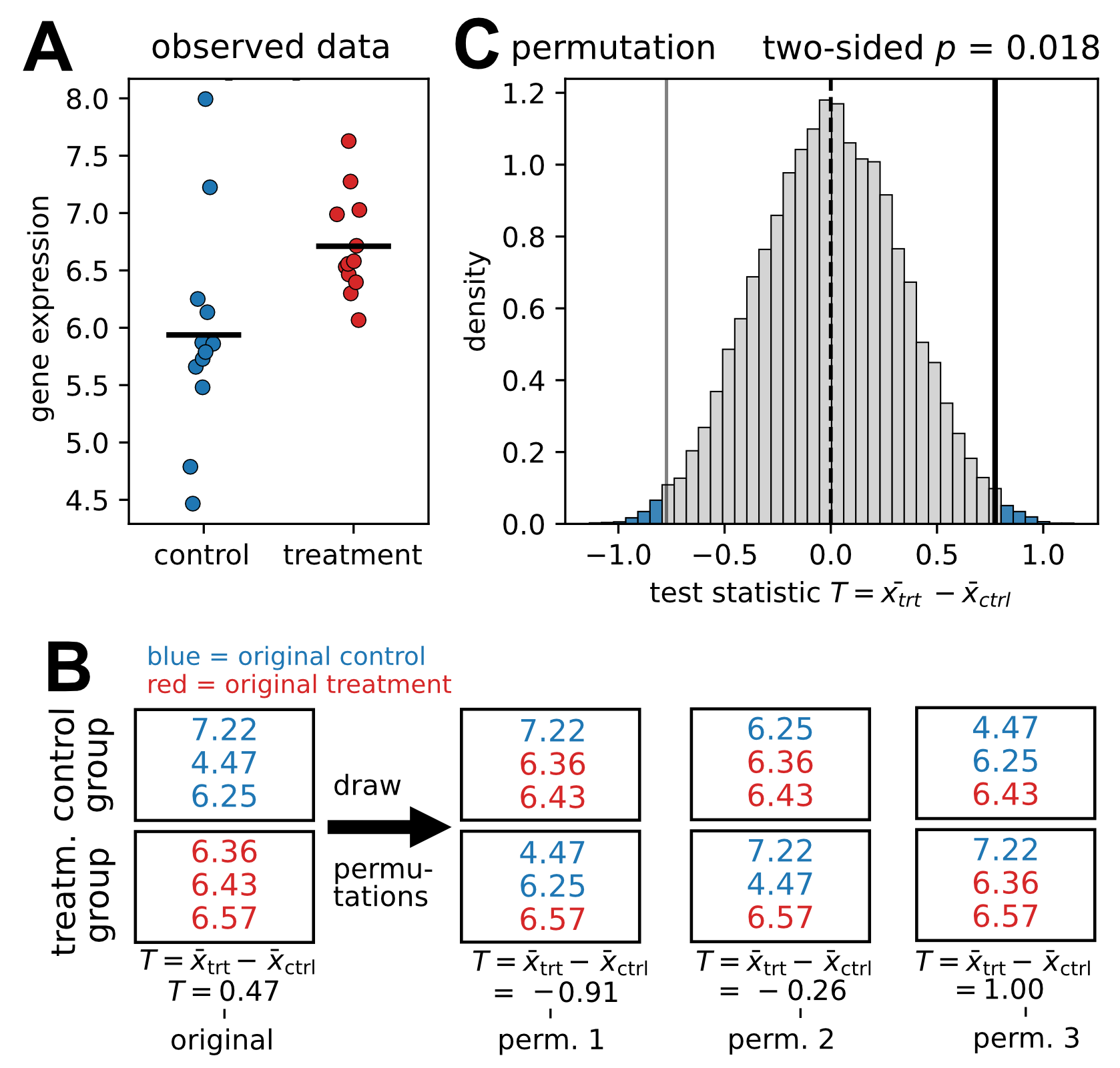
A canonical example is gene expression analysis. Suppose we measure the expression level of a gene across multiple biological replicates in two conditions, for example untreated cells and cells exposed to a drug. Each condition yields a set of expression measurements, and we observe that the average expression differs between groups (Fig. 13.2A).
At this stage, two distinct questions arise:
How large is the observed difference?
Is the difference signficiant or could a difference of this size plausibly arise if the drug had no effect?
The first question concerns effect size and uncertainty, which we can quantify using e.g. SEMs or bootstrapping. The second question requires a hypothesis test.
The null hypothesis in this setting is: Expression measurements in the two conditions are drawn from the same underlying distribution.
13.4 Permutation tests to evaluate differences
Importantly, this null hypothesis does not specify a particular probabilistic model or probability distribution for expression values. Instead, it states that the experimental condition does not influence expression. If this is true, then the labels “control” and “treatment” are arbitrary and carry no information. In other words, under the null-hypothesis, the assignment of measurements to conditions is interchangeable. But if that is true, then randomly reassigning condition labels should not systematically change the observed difference in expression. To evaluate the null-hypothesis we thus run a permutation test. That is, we randomly assign measurements to different conditions and examine the consequences for a statistic of interest. Specifically, to perform a permutation test, we proceed as follows:
Compute the observed test statistic of interest, for example the difference in mean expression between conditions.
Randomly assign the measured expression levels to the condition labels. Figure 13.2B shows, as simplified example, a few permutations for 6 datapoints only.
Recompute the test statistic for the shuffled data.
Repeat this procedure many times to generate a reference distribution under the null hypothesis.
Compare the observed test statistic to this distribution to obtain a p-value.
For the data in Figure 13.2A the result of the permutation test is shown in Figure 13.2C. Technically, it shows the null distribution obtained by permuting condition labels many times. The blue shaded region indicates permutation outcomes at least as extreme as the observed difference and defines the p-value. For this example, the resulting p-value is 0.018, meaning that under the typical threshold of 0.05 we do consider the gene expression levels to be significantly different.
13.5 Relation to classical parametric tests
Notably, permutation tests like the one shown construct the null distribution directly from the data. Permutation tests therefore provide a powerful and general framework for hypothesis testing in biological data, especially when analytical distributions are unknown or unreliable. Historically, however, parametric tests, most commonly the t-test, have been widely used in biological data analysis. These tests are elegant and powerful when their assumptions are satisfied, but they rely on key assumptions such as independent observations, approximately normally distributed noise, and similar variances between groups.
Biological data frequently violate these assumptions, in which case parametric p-values can become misleading. In many biological settings, permutation tests are therefore preferable, as they make fewer assumptions and rely directly on the structure of the observed data.
The t-test is one of the most widely used statistical tests in the life sciences and has been a cornerstone of data analysis for more than a century. It was introduced by William Sealy Gosset in 1908, working under the pseudonym Student, to address inference from small-sample experiments when the population variance is unknown.
At the time, computation was done by hand and analytical solutions were essential. The t-test provided a simple, closed-form way to assess whether two group means differ more than expected from sampling variability alone. For much of the 20th century, it became the default tool for hypothesis testing in biology, medicine, and the social sciences.
From a modern perspective, the t-test can be understood as a special case of a more general idea: it approximates the sampling distribution of a difference in means under the assumptions of independent observations, approximately Gaussian noise, and similar variances between groups. When these assumptions hold, the t-test is powerful.
However, it is now feasible with modern computers to construct null distributions directly from the data using permutation tests. Permutation tests require fewer assumptions, make the null hypothesis explicit, and work naturally for arbitrary test statistics and small sample sizes. Thus, while the t-test remains useful and interpretable under its assumptions, permutation tests provide a more general and transparent framework for hypothesis testing in contemporary biological research.
| Feature | t-test | Permutation test |
|---|---|---|
| Distribution assumptions | Yes | No |
| Small sample sizes | Risky | Robust |
| Arbitrary test statistics | No | Yes |
13.6 Practical implementation and important caveats
With modern computational tools, permutation tests are straightforward to implement. We show how this is done in Python in Problem Set 5. However, it is important to recognize that hypothesis testing and p-values come with important limitations and potential pitfalls.
A p-value is not the probability that the null hypothesis is true. It is the probability of observing data at least as extreme as those measured, assuming the null hypothesis is true.
A small p-value does not measure effect size or biological relevance. Statistical significance does not imply biological importance.
Significance thresholds are arbitrary. Common cutoffs such as \(p<0.05\) are conventions, not fundamental scientific boundaries.
P-values alone do not establish biological hypotheses. Robust conclusions require independent validation, additional data, and complementary experiments. Hypothesis testing does not replace the need for clever experimental design and rigerous research.
Multiple hypothesis testing must be accounted for. When many tests are performed, false positives accumulate unless appropriate corrections are applied.
We discuss multiple hypothesis testing and correction methods in detail in the next section.