17 Nonlinear dimensionality reduction and UMAP
In many datasets, variation is structured along curved or branching manifolds that cannot be well approximated by a linear subspace. In such cases, nonlinear methods can be useful. A widely used example is UMAP (Uniform Manifold Approximation and Projection), which is based on ideas from topology and manifold learning.
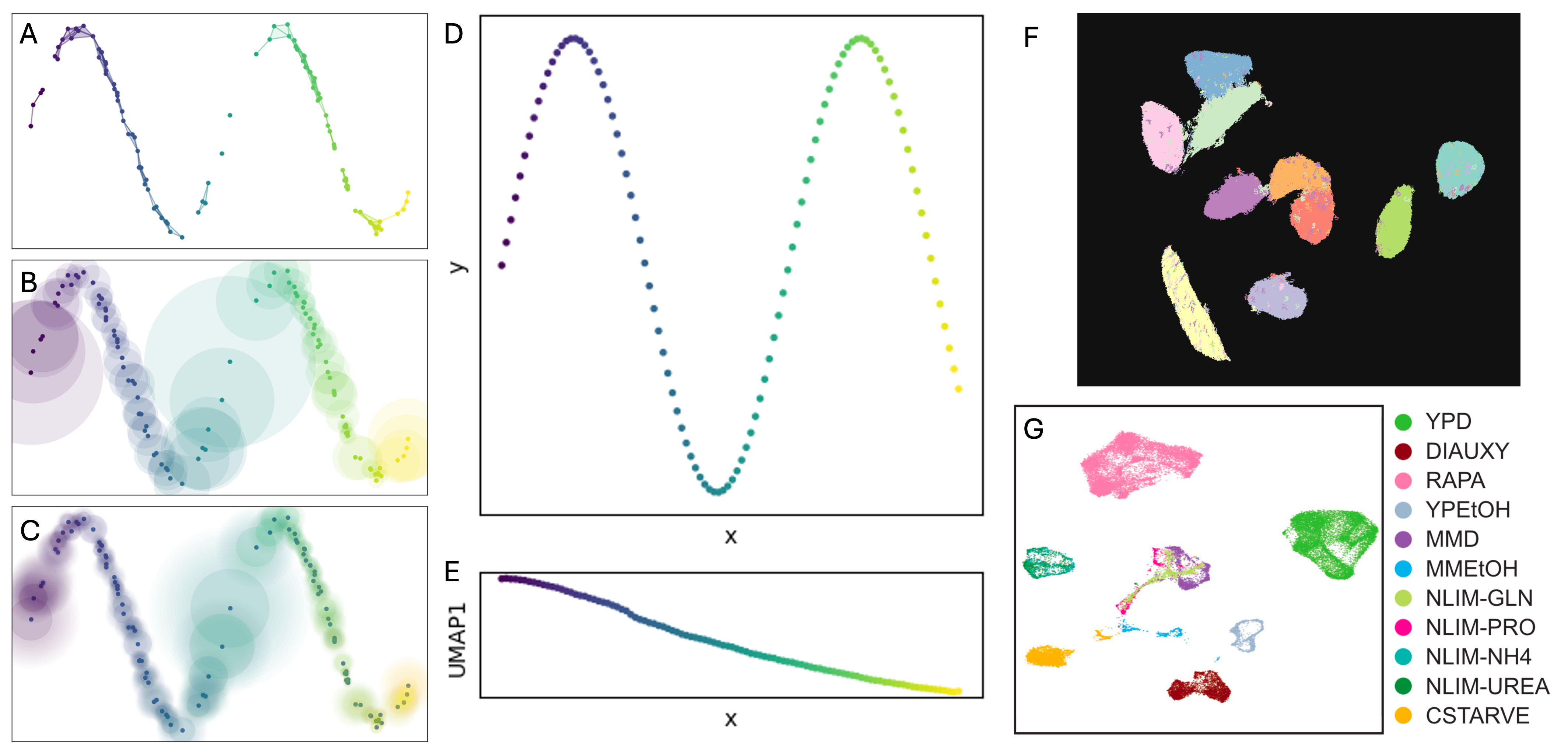
Constructing a neighborhood graph: UMAP starts by identifying, for each data point, its \(k\) nearest neighbors in the original high-dimensional space (typically using Euclidean or cosine distance). From these neighbors, UMAP builds a weighted graph in which:
nodes represent samples,
edges connect neighboring samples,
edge weights reflect how close two samples are.
These weights are chosen so that nearby points are connected with high probability, while distant points are weakly connected. This graph represents the local geometry of the data.
Interpreting neighborhoods as fuzzy sets: UMAP interprets each local neighborhood as a fuzzy set, meaning that membership is gradual rather than binary. Two points can be connected strongly, weakly, or not at all. All local fuzzy neighborhoods are then combined into a single global fuzzy graph that approximates the manifold structure of the data. This step encodes the assumption that the data lie on a low-dimensional manifold embedded in high-dimensional space.
Low-dimensional embedding: UMAP then seeks a low-dimensional representation (typically 2D or 3D) in which the distances between points reproduce the structure of the fuzzy graph as closely as possible. Formally, UMAP constructs a similar fuzzy graph in the low-dimensional space and optimizes the embedding by minimizing a cross-entropy loss between the high- and low-dimensional graphs. This optimization balances two competing goals:
nearby points in high dimensions should remain close,
unrelated points should be separated.
The result is an embedding that preserves local neighborhoods while arranging them coherently in low dimensions. For further details, discussion and examples for how to implement UMAP we recommend the documentation and accompanying tutorials at https://umap-learn.readthedocs.io.
Interpretation and limitations: Unlike PCA, UMAP does not produce linear axes or interpretable coefficients. The embedding coordinates have no direct physical meaning. UMAP is also stochastic: different runs may yield slightly different layouts unless random seeds are fixed. Because UMAP emphasizes local structure, distances between far-apart clusters are not necessarily meaningful. Apparent cluster separation or trajectories should therefore be interpreted cautiously and ideally validated by independent biological information.