21 Stochastic Processes
Optional topic. Weeks 8 and 9 (dynamical systems and nonlinear dynamics) are an optional part of the course.
Differential equations, such as those introduced earlier to model the central dogma, are powerful tools for analyzing dynamical systems. However, by construction, models based on differential equations are deterministic. That is, once the initial condition is specified, the trajectory is entirely determined by the governing equation. For a fixed initial condition, there is no variability in the predicted dynamics.
Real biological processes, however, are noisy and fluctuate in time. This naturally raises the question of how appropriate a purely deterministic description is for modeling biological systems, and whether a probabilistic framework might sometimes be more suitable. This is not merely a technical complication; stochasticity is a fundamental feature of biology, and in many cases it plays a central role in how cells function and make decisions.
As an example, consider the transcription and translation dynamics of a gene in a bacterial cell, as discussed in the previous section. We estimated typical mRNA copy numbers to be very low, on the order of one molecule per cell. In this regime, dynamics are not smooth and continuous but instead consist of discrete stochastic events. Relative fluctuations are large, as a change of just one or two molecules represents a substantial fraction of the mRNA copy number. Consequently, gene expression in bacteria is inherently stochastic, and this stochasticity propagates through translation, leading to variability in protein levels.
To analyze such situations more systematically, we now introduce the basic concepts of stochastic processes.
21.1 The Poisson Process
We start with a simple stochastic process. We study a random variable \(N(t)\) that increases by one whenever a new event occurs, with the key characteristic that events occur with a constant probability per unit time, denoted by the rate \(k\). Mathematically, the probability that an event occurs during a short time interval \(\Delta t\) is
\[\mathbb{P}(\text{one event in } \Delta t) = k \, \Delta t,\]
while the probability of two or more events during \(\Delta t\) is negligible for sufficiently small \(\Delta t\). This assumption defines a Poisson process, and we will see below why it is called that way.
To describe the occurring dynamical process mathematically, we introduce the probability \(P(N,t)\) that the system is in state \(N\) at time \(t\). Events increase \(N\) by one, so probability flows from state \(N-1\) into \(N\). The time evolution of \(P(N,t)\) is therefore governed by the equation
\[\frac{dP(N,t)}{dt} = k \, P(N-1,t) - k \, P(N,t).\]
The first term represents transitions into state \(N\), while the second term represents transitions out of state \(N\). This equation is an example of a master equation.
In general, master equations are difficult to solve analytically. However, we can simulate stochastic trajectories numerically. Instead of computing \(P(N,t)\) directly, we repeatedly generate sample paths by letting the computer draw random variables to determine when the next event occurs and updating \(N\) accordingly. To do so, we must know the probability distribution of the waiting time until the next event.
For a Poisson process, the waiting time \(\tau\) between events follows an exponential distribution,
\[p(\tau) = k \, e^{-k \tau},\]
as derived in the box below. Drawing \(\tau\) from this distribution and updating the system step by step yields one realization of the stochastic trajectory.
We derive the probability distribution of the waiting time \(\tau\) until the next event occurs in a Poisson process with constant rate \(k\).
Let \(P_{ne}(t)\) denote the probability that no event has occurred up to time \(t\). During a short interval \(\Delta t\), the probability that no event occurs is \[1 - k \Delta t\] .
Therefore, \[P_{ne}(t+\Delta t) = P_{ne}(t)\,(1 - k \Delta t).\]
Rearranging gives \[\frac{P_{ne}(t+\Delta t) - P_{ne}(t)}{\Delta t} = -k\, P_{ne}(t).\]
Taking the limit \(\Delta t \to 0\) yields the differential equation \[\frac{dP_{ne}}{dt} = -k\, P_{ne}(t).\]
This equation has the solution \[P_{ne}(t) = e^{-k t},\] using the initial condition \(P_{ne}(0)=1\) (no even occurred at time \(t=0\) by definition).
What is the probability that the next event occurs exactly at time \(\tau\)?
Intuitively, two things must happen:
1. No event occurs before time \(\tau\). 2. An event occurs immediately after time \(\tau\).
The probability that no event has occurred before \(\tau\) is \[P_{ne}(\tau) = e^{-k\tau}.\]
The probability that an event occurs in the next small interval \([\tau, \tau+\Delta t]\) is approximately \(k \Delta t\).
Therefore, the probability that the event occurs between \(\tau\) and \(\tau+\Delta t\) is \[P_{ne}(\tau)\, k \Delta t.\]
Dividing by \(\Delta t\) and taking the limit \(\Delta t \to 0\) gives the probability density \[p(\tau) = k e^{-k\tau}.\]
Thus, the waiting time between events in a Poisson process follows an exponential distribution.
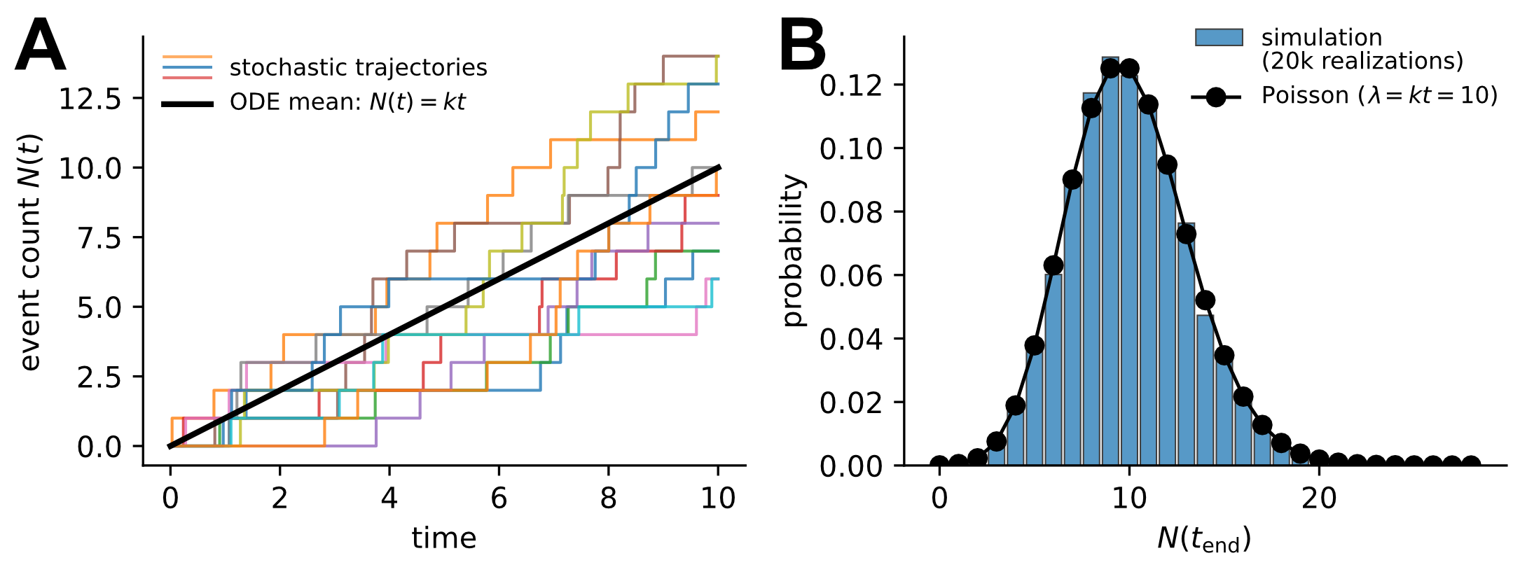
An example of stochastic trajectories generated in this way is shown in Fig. 21.1A. Each trajectory (or realization of the stochastic process) consists of discrete jumps occurring at random times. Importantly, repeating the simulation produces different trajectories, reflecting the inherent stochasticity of the process.
By generating many independent realizations, we can explore the statistical properties of the system. For example, we can examine the distribution of \(N(t)\) at a fixed time point, as shown in Fig. 21.1B.
Notably, this distribution follows a Poisson distribution,
\[P(N,t) = \frac{(k t)^N}{N!} e^{-k t},\]
(black line in Fig. 21.1B), which explains the name Poisson process: not only are the waiting times exponentially distributed, but the total number of events occurring in a fixed time interval follows a Poisson distribution.
Intuitively, this result can be understood by dividing time into many small intervals \(\Delta t\). In each interval, an event occurs with probability \(k \Delta t\), analogous to repeatedly flipping a highly biased coin. The total number of events in time \(t\) then follows a binomial distribution, which converges to a Poisson distribution in the limit \(\Delta t \to 0\).
21.2 The Gillespie Algorithm
To study biologically relevant situations, we must go beyond a single Poisson process. The Poisson process resembles, in the deterministic limit, the simple differential equation
\[\frac{dN}{dt} = k,\]
which describes a constant production rate. Real biological systems, however, typically involve multiple interacting processes whose rates depend on the current state of the system. For example, in exponential growth we have
\[\frac{dN}{dt} = \lambda N,\]
so the rate of events depends on the current population size. Similarly, in gene expression, transcription, translation, and degradation occur simultaneously, and their rates depend on molecule numbers.
To formalize this idea, we introduce the concept of a propensity. The propensity \(a_j(x)\) of reaction \(j\) is the probability per unit time that this reaction occurs, given the current state \(x\) of the system. Importantly, propensities depend on molecule numbers. For example, the degradation of mRNA occurs at a rate proportional to the number of mRNA molecules present. If twice as many molecules are present, twice as many degradation events are expected per unit time. In this sense, propensities represent the stochastic analogue of reaction rates in differential equations.
To simulate such systems stochastically, we use the Gillespie algorithm, introduced by Daniel Gillespie. This algorithm provides an exact simulation method for chemical master equations. The core idea is simple: given the current state of the system, we calculate the rates at which all possible reactions can occur, and then use two random numbers to determine (i) when the next reaction occurs and (ii) which reaction it is. See the box for more details.
The Gillespie algorithm provides an exact simulation method for stochastic chemical reaction systems described by a master equation.
Consider a system with reactions \(j = 1, \dots, R\). Each reaction has a propensity \(a_j(x)\), defined as the probability per unit time that reaction \(j\) occurs given the current state \(x\) of the system.
Step 1: Compute propensities.
For the current state, compute all propensities \(a_j\) and their sum \[a_0 = \sum_{j=1}^R a_j.\]
Step 2: Draw time to next reaction.
The waiting time \(\tau\) until the next reaction is drawn from an exponential distribution with rate \(a_0\): \[\tau = \frac{1}{a_0} \ln\!\left(\frac{1}{u_1}\right),\] where \(u_1 \in (0,1)\) is a uniform random number.
Step 3: Choose which reaction occurs.
Select reaction \(j\) such that \[\sum_{i=1}^{j-1} a_i < u_2 a_0 \le \sum_{i=1}^{j} a_i,\] where \(u_2 \in (0,1)\) is a second independent uniform random number. This selects reaction \(j\) with probability \(a_j / a_0\).
Step 4: Update the system.
Update the system state according to the stoichiometry of reaction \(j\) and advance time by \(\tau\).
Step 5: Repeat.
Return to Step 1 and iterate.
This procedure generates statistically exact trajectories of the underlying chemical master equation and is the standard method for simulating low-copy-number stochastic systems such as gene expression.
21.3 Stochastic Gene Expression: The Central Dogma Revisited
To illustrate how stochastic simulation can be applied to a biologically relevant system, we now revisit the central dogma model previously introduced in deterministic form. Specifically, we described earlier the mRNA and protein dynamics using differential equations, \[\frac{dm}{dt} = G\kappa - \delta_m m, \qquad \frac{dp}{dt} = \gamma m - (\delta_p+\lambda) p,\] where \(\kappa\) is the transcription rate, \(\delta_m\) the mRNA degradation rate, \(\gamma\) the translation rate per mRNA, and \(\delta_p\) and \(\lambda\) the protein degradation and dilution rate due to growth.
In the stochastic formulation, we no longer track continuous concentrations, but instead integer molecule numbers \(m\) and \(p\). Changes occur through four discrete reaction events:
| Transcription: | \(m \rightarrow m+1\) with propensity \(G\kappa\) |
| mRNA degradation: | \(m \rightarrow m-1\) with propensity \(\delta_m m\) |
| Translation: | \(p \rightarrow p+1\) with propensity \(\gamma m\) |
| Protein removal: | \(p \rightarrow p-1\) with propensity \((\delta_p+\lambda) p\) |
These reactions define a chemical master equation, which we simulate using the Gillespie algorithm. That is, we determine the total rate at which any of the four reactions occurs by summing their propensities, then use one random number to determine the time of the next event and a second random number to determine which reaction occurs.
Stochastic trajectories.
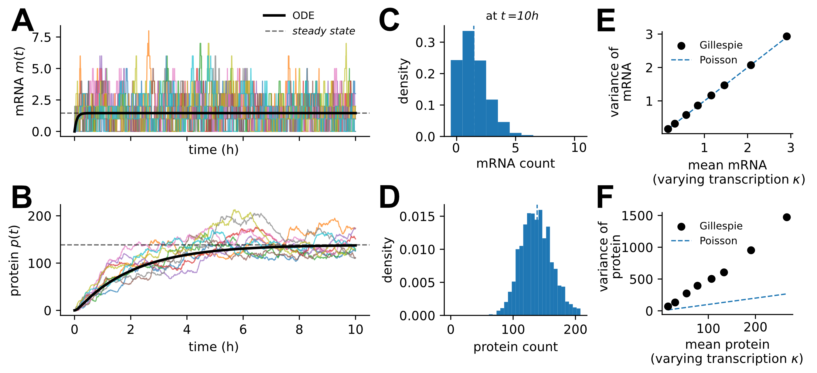
Simulating this system produces stochastic trajectories for \(m(t)\) and \(p(t)\). As an example, we consider induction of gene expression starting from low copy numbers. The resulting trajectories are shown in Fig. 21.2A and B for mRNA and protein copy numbers, respectively. Each line represents one realization of the stochastic process. Unlike the smooth deterministic solution, these trajectories exhibit discrete jumps and fluctuations.
Importantly, the trajectories fluctuate around the deterministic steady states, \[m^* = \frac{G\kappa}{\delta_m}, \qquad p^* = \frac{\gamma m^*}{\delta_p+\lambda},\] which were derived in the previous section. The deterministic differential equations therefore describe the mean behavior of the system, while the stochastic simulations reveal the variability around that mean.
Steady-state distributions and noise scaling.
To characterize this variability in more detail, we analyze the distribution of copy numbers once the system has reached steady state. Figures 21.2C and D show the steady-state distributions of mRNA and protein counts across many independent realizations.
We can further quantify noise by analyzing how the variance scales with the mean. To this end, we vary the transcription rate \(\kappa\) while keeping all other parameters fixed. For mRNA, the variance scales approximately linearly with the mean (Fig. 21.2E), as expected for a Poisson process where \[\mathrm{Var}(m) = \langle m \rangle.\]
In contrast, the variance of protein copy numbers increases faster than the mean (Fig. 21.2F), indicating overdispersion relative to a Poisson process. This enhanced variability arises because protein synthesis depends on the stochastic mRNA copy number. Fluctuations in mRNA propagate to proteins and effectively amplify noise. Protein dynamics therefore combine intrinsic stochasticity in translation with inherited fluctuations from upstream transcriptional events.
21.4 Transcriptional Bursting
Overall, these considerations suggest a considerable amount of noise in gene expression. However, in real cells gene expression noise can be even stronger than predicted by this minimal birth–death model. In both bacteria and eukaryotes, genes are often not transcribed at a constant rate but rather in bursts: periods of high transcriptional activity alternate with silent periods. This phenomenon, known as transcriptional bursting, arises from stochastic switching of promoters between active and inactive states.
This produces mRNA distributions that are broader than Poisson. Notably, this is consistent with the overdispersion often observed in RNA-seq data. The negative binomial distribution commonly used to model RNA-seq counts can be interpreted as the steady-state distribution expected from a bursting gene. In practice, however, negative binomial dispersion estimates in differential expression tools such as DESeq2 may also reflect additional sources of variability, including biological heterogeneity and measurement noise.