14 Multiple hypothesis testing
Hypothesis testing becomes particularly challenging when many hypotheses are tested simultaneously. This situation is common in modern biological research, especially in high-throughput and exploratory studies such as transcriptomics, proteomics, genome-wide association studies, and large-scale screens, where thousands to millions of tests may be performed in parallel.
In this setting, naive interpretation of p-values can be highly misleading. For example, if we test 10,000 independent hypotheses, then even if all null hypotheses are true, a common significance threshold of \(\alpha = 0.05\) implies that we expect on average about 500 false positives purely due to random variation.
The core challenge is that p-values are defined for a single hypothesis test. When many tests are performed, the probability of observing small p-values increases. This is not a flaw of statistics, but a mathematical consequence of repeated testing.
In modern biological settings, this problem is especially acute because:
datasets are large and high-dimensional,
many hypotheses are tested, often generated post hoc,
measurements are noisy and heterogeneous,
follow-up experiments are costly.
How can we deal with this challenge and prevent large numbers of false discoveries that misdirect resources and obscure true biological signals?
14.1 Error rates and false positives
To understand how multiple testing corrections work, it is useful to introduce formally false positives and error rates.
[TABLE]
A case in which a test is declared significant when the null hypothesis is in fact true is called a false positive, or a Type I error. The probability of making such an error in a single test is controlled by the significance level \(\alpha\). For a single hypothesis test, using \(\alpha = 0.05\) means that we accept a 5% chance of a false positive.
When \(m\) hypotheses are tested simultaneously, the expected number of false positives is approximately \[m \alpha.\] Thus, even moderate values of \(\alpha\) can lead to large numbers of false discoveries in large-scale studies.
Two major error rates are commonly used to control this problem:
Family-wise error rate (FWER).
The family-wise error rate is the probability of making at least one false positive among all tests. A classical method to control the FWER is the Bonferroni correction, which replaces \(\alpha\) with \[\alpha_{\mathrm{Bonf}} = \frac{\alpha}{m}.\] Only p-values smaller than \(\alpha/m\) are declared significant. This approach is simple and rigorous, but often overly conservative in large datasets.
Suppose we perform \(m\) independent hypothesis tests, each at significance level \(\alpha'\). Let’s assume the worst case: each hypothesis test is a true null, and let’s call each hypothesis test \(\mathcal{H}_0^{(1)}, \mathcal{H}_0^{(2)}, ... , \mathcal{H}_0^{(n)}\).
For a single test, the probability of a false positive is at most \(\alpha'\).
The probability of at least one false positive across all tests satisfies \[\mathbb{P}(\text{at least one false positive}) \le m \alpha'.\]
To see this we use the union bound:
\[\begin{align*} & \mathbb{P}(\text{at least one false positive}) \\ = & \mathbb{P} (\{\text{reject }\mathcal{H}_0^{(1)} \} \cup \{ \text{reject} \mathcal{H}_0^{(2)} \} \cup .. \cup \{ \text{reject} \mathcal{H}_0^{(n)} \})\\ \leq & \mathbb{P} (\{\text{reject }\mathcal{H}_0^{(1)} \}) + ... + \mathbb{P} (\{\text{reject }\mathcal{H}_0^{(n)} \}) = m\alpha' \end{align*}\]
To ensure that this probability is at most \(\alpha\), we require \[m \alpha' \le \alpha.\]
We can see that if \(\alpha' = \frac{\alpha}{m}\), the above condition is met.
This leads to the Bonferroni correction: each individual test is evaluated at level \(\alpha/m\), guaranteeing control of the family-wise error rate.
False discovery rate (FDR).
The false discovery rate is the expected fraction of false positives among all rejected hypotheses. Controlling the FDR allows some false positives, but limits their proportion. Referring to the table above, \(FDR = V/R\); the number of false discovery per rejected null hypothesis. Procedures such as the Benjamini–Hochberg method adaptively adjust p-value thresholds and are widely used in omics and screening studies.
FDR control typically provides a better balance between discovery and reliability in exploratory biological research. This is ideal for finding candidate effects, where tolerance for false positives is higher.
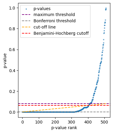
The Benjamini–Hochberg (BH) method controls the false discovery rate (FDR) by comparing each p-value to an adaptive threshold.
Let \(p_{(1)} \le p_{(2)} \le \dots \le p_{(m)}\) be the sorted p-values.
For a desired FDR level \(q\), BH finds the largest index \(k\) such that \[p_{(r)} \le \frac{r}{m} q.\]
This is visualized below, on a plot showing p-values arranged by rank.
The procedure is as follows:
Sort p-values into ascending order.
Find the largest p-value (\(p_{(k)}\)) that meets the condition \(p_{(r)} \leq \frac{rq}{m}\)
Reject the null hypothesis for all values lower than \(p_{(r)}\)
See the box below for the proof for why this controls FDR at level \(q\).
The goal of the procedure above, which we will show here that it meets, is to bound the expected FDR at a level \(q\) (commonly set to 0.05). Referring to the table showing different types of error rates above, this is equivalent to wanting \[\text{FDR} = V/R \leq q.\]
The orange line in Figure 14.1 represents the maximum value p-value which would satisfy keeping the expected FDR bounded by \(q\). This is a linear relationship because the FDR is the ratio between total hypotheses rejected and allowable false positives; as we reject more hypothesis, we’re comfortable with proportionally more false discoveries.
Let’s remember that p-values arising from true null hypotheses are uniformly distributed between 0 and 1; \(p \sim \text{Uniform}(0,1)\), or equivalently \(\mathbb{P}(p \leq t) = t\) for \(t \in [0,1]\).
For the Benjamini-Hochberg procedure, all rejected p-values satisfy \(p_{(i)} < \frac{rq}{m}\), where \(r\) is the total number of rejected hypotheses, \(q\) is the level at which FDR is controlled, and \(m\) is the total number of tests. To see this visually, remember that we reject all p-values up until rank \(r\) that are under the line \(y = x \frac{q}{m}\); \(\frac{q}{m}\) is the slope (you can see this as this is the maximum distance in the orange line divided by the maximum x-distance). Let’s call this bound on p-values of rejected hypotheses \(t_r := \frac{rq}{m}\).
From following the procedure on the data, we now have a fixed value for; \(R = r\). Let’s call the number if true nulls in the data (which we cannot measure) \(m_0\). The probability of a true null having a p-value below \(t_r\) is simply \(t_r\), so the expected number of true nulls (i.e E(V)) below \(t_r\) is \(t_rm_0\).
by substituting this into the definition of FDR, we can see that the expected value of FDR is indeed bounded by \(q\):
\[E \bigg[\frac{V}{R} \bigg] = \frac{t_rm_0}{r} = \frac{rqm_0}{mr} = q \frac{m_0}{m} \leq q.\]
14.2 Final notes
Multiple-testing correction does not turn hypothesis testing into a definitive decision rule. Even after correction, a small p-value only indicates that the data are unlikely under a specified null model; it does not establish biological truth.
In biology, hypothesis testing should therefore be viewed as a tool for prioritization rather than confirmation. Statistical significance helps identify candidates for follow-up, but robust conclusions require independent data, replication, and mechanistic understanding.
This point will be emphasized when we specifically consider omics data and their biological interpretation.