10 A probabilistic view and the law of large numbers
Following data visualization and fitting (regression), a common next step is to evaluate results and assess their reliability. This requires a quantitative analysis of uncertainty, which in turn requires statistical considerations.
10.1 Measurements as random variables
As discussed previously, biological data are inherently variable, reflecting a combination of biological heterogeneity, technical noise, and procedural effects (see Section 4). As a consequence, repeated measurements under identical experimental conditions do not produce identical numerical outcomes. We therefore need to adopt a probabilistic perspective.
Key to a probabilistic description is treating measurement results not as fixed values, but as random variables drawn from an underlying probability distribution. A single measurement provides one realization from this distribution, not a direct measurement of the true underlying biological quantity. Repeating the same experiment under identical conditions produces not a single number, but a distribution of values. It is this distribution that contains the information we seek, and statistical quantities such as means or standard deviations summarize properties of this distribution and our uncertainty about it.
A random variable is a quantity whose value can vary between repeated measurements, even when experimental conditions are kept the same. We denote a random variable by a symbol such as \(X\).
A probability distribution describes how likely different values of \(X\) are to occur. For a discrete variable, this is specified by probabilities \(P(X = x)\); for a continuous variable, by a probability density \(p(x)\). Probability distributions are normalized such that the total probability equals one.
To illustrate this probabilistic perspective, consider a coin-toss experiment. Suppose a coin lands heads with probability \(p\) and tails with probability \(1-p\). A single coin toss produces one outcome—heads or tails—but this single observation does not tell us much about the underlying process (for example, how large \(p\) is).
In technical terms, a single toss is one sample from the underlying probability distribution, but it is insufficient to characterize that distribution. By repeating the coin toss many times, we obtain a collection of outcomes whose relative frequencies allow us to estimate the underlying probability \(p\). This illustrates a general principle: repeated measurements allow us to learn about the properties of an underlying probability distribution.
The coin-toss experiment is one of the few cases where the probability distribution and its statistical properties can be treated fully analytically. Each toss follows a Bernoulli process. Most biological experiments are more complex: the underlying distributions are rarely known exactly and are often analytically intractable. Accordingly, numerical approaches play a central role in biological data analysis, including for the coin-toss example discussed here.
10.2 The law of large numbers
A particularly important property of a probability distribution is its mean, also called the expected value. The mean provides a central tendency of the distribution and is often the quantity of biological interest.
The mean (or average) of a random variable describes the central value of its underlying probability distribution.
For a discrete random variable \(X\) that takes values \(x\) with probabilities \(P(X=x)\), the mean is defined as \[\mu = \sum_x x\, P(X=x).\]
For repeated measurements \(X_1, X_2, \dots, X_n\), the corresponding sample mean is \[\bar{X}_n = \frac{1}{n} \sum_{i=1}^{n} X_i.\]
For the coin-toss example, we can assign the value \(X=1\) to heads and \(X=0\) to tails. The sample mean of many coin tosses then corresponds to the fraction of heads observed (Fig. 10.1A). Importantly, as the number of coin tosses increases, the sample mean stabilizes and approaches the true probability \(p\) of obtaining heads. This behavior is illustrated in Fig. 10.1B using computational simulations of repeated coin tosses. Notably, the convergence occurs despite each individual outcome remaining random. This fundamental behavior is known as the law of large numbers.
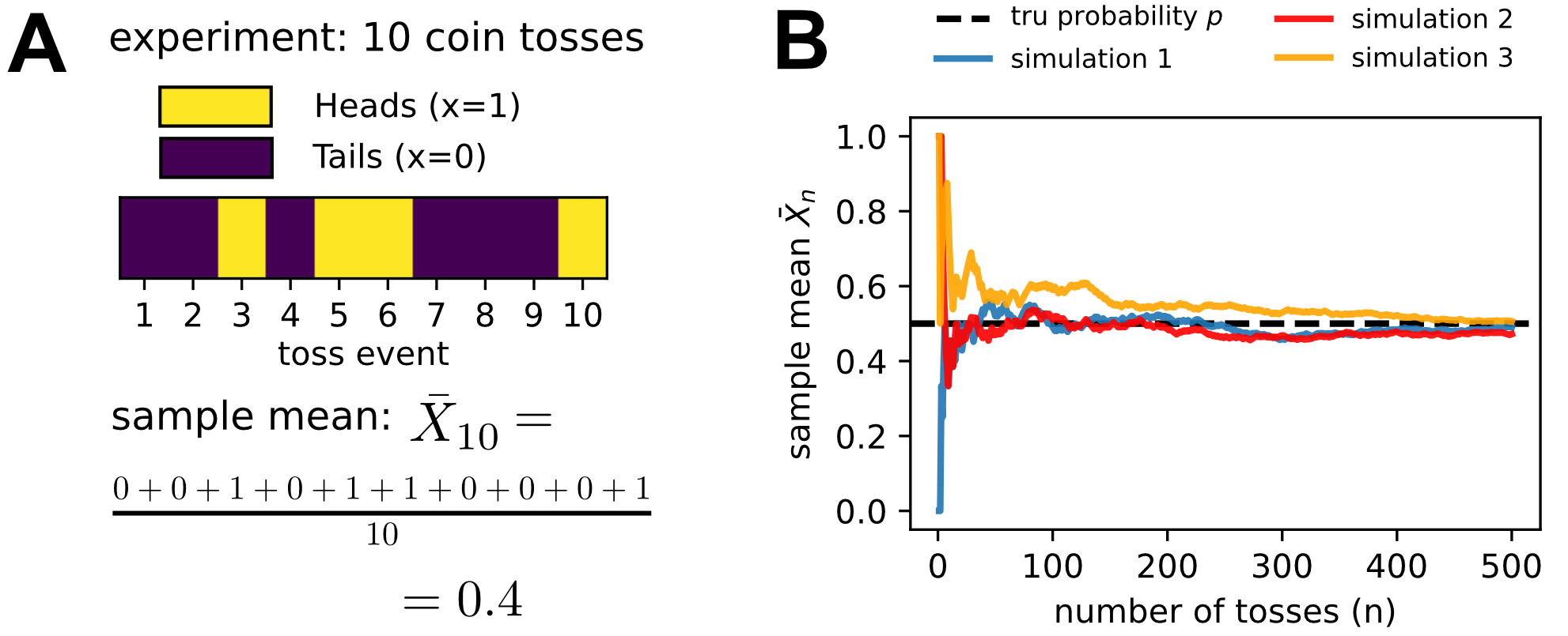
For independent and identically distributed random variables with a finite expected value, the sample mean converges to the true expected value as the number of observations increases.
The importance of the law of large numbers is hard to overstate. It provides the theoretical foundation for estimating average biological quantities through repeated measurements and explains why increasing sample size improves the reliability of experimental results.
Crucially, the law of large numbers relies on assumptions. Measurements must be independent and drawn from the same underlying distribution. In biological experiments, these assumptions are often—but not always—satisfied as outlined more in the box.
The assumptions underlying the law of large numbers can be violated in biological experiments. Particularly, independence might not be ensured. Batch effects can introduce systematic shifts between measurements, time correlations can arise in longitudinal studies, and shared reagents or instruments can induce dependencies between samples. Recognizing these effects and designing experiments to minimize them is essential for correct statistical interpretation.
Together, while variability is unavoidable in biology, repeated measurements allow us to extract robust quantitative insights about expectation values. In the following sections, we build on this probabilistic foundation to introduce uncertainty estimates, beginning with the standard error of the mean.