18 Clustering Algorithms
As we’ve seen so far, high-dimensional (or other) data can often form sub-groups or clusters. Common instances of these include groups based on environmental condition, developmental state, cell type or state, samples from geographic locations, batch effects, etc. These show up intuitively in visualizations, but can actually be non-trivial to automatically group into clusters. There is a very large family of algorithms, which each have different use cases. Here we discuss the canonical examples of k-means in some depth, and provide a brief overview of other examples. Most standard clustering algorithms are easily implemented with standardized and efficient packages across common coding languages.
K-means clustering
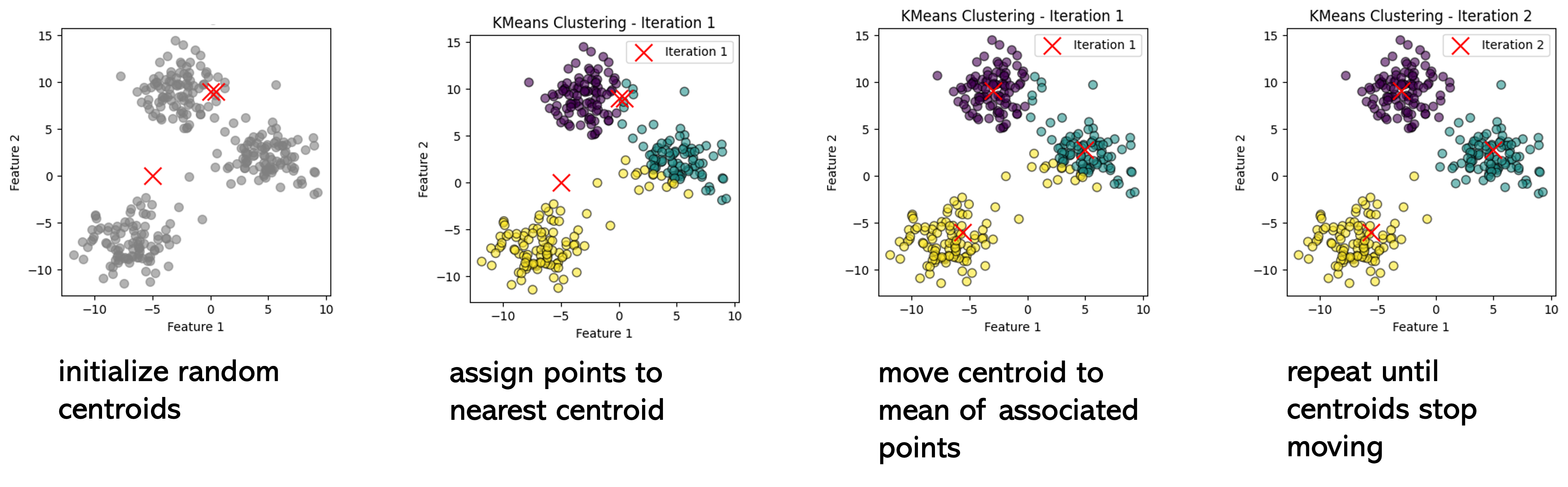
The K-means algorithm is as follows:
Initialize centroids randomly. The number of centroids is pre-determined and corresponds to the number of clusters.
Assign each point to the nearest centroid.
Move each centroid to the mean location of the points in the cluster
Repeat until the algorithm converges and points no longer change assignments
Note that it is possible for this algorithm to get stuck in a “pathological" state, where centroids end up not at the center of intuitive (or optimal) clusters, but rather at points in between clusters of datapoints. This is conceptually similar to getting stuck at a local minimum in optimization methods we have discussed so far. To avoid this, it is useful to visualize the clusters to verify that they make sense intuitively, to repeat the algorithm with a few iterations of initial locations for the cluster centroids.
Beyond k-means, there are many other clustering methods that can handle situations where its assumptions are too restrictive. Hierarchical clustering, for example, builds a tree of clusters by either repeatedly merging small groups into larger ones or splitting large groups into smaller ones, allowing us to view the data at different levels of detail. Density-based methods such as DBSCAN group together points that lie in crowded regions and mark isolated points as noise, which makes them useful for finding irregularly shaped clusters. Another approach models the data as coming from a mixture of distributions and uses the Expectation–Maximization algorithm to estimate which points likely belong to which group, allowing for partial membership rather than forcing each point into a single cluster. There are also graph-based and spectral methods that rely on measuring how similar points are to one another to uncover more complex patterns. The figure below adapted from this blog shows how different algorithms perform in different contexts.
Finally, take care when interpreting the results of clustering. Many clustering algorithms involve some degree of randomness—for example, different initial starting points can lead to different solutions—so repeated runs may not produce identical groupings. In addition, results can change substantially depending on choices such as the number of clusters, distance measure, or tuning parameters (for instance, the neighborhood size in DBSCAN). For this reason, it is good practice to check the stability of clusters under different settings and to consider whether the solution is consistent with domain knowledge.
It is also important to remember that most clustering algorithms will produce clusters even if the data do not contain any meaningful grouping. The presence of clusters in the output does not by itself prove that a strong or “real” cluster structure exists; apparent groupings may arise from noise, scaling choices, or high dimensionality. Whenever possible, clustering results should be supported with additional evidence, such as external validation, replication on new data, or quantitative measures of stability.
Finally, be cautious when clustering points based on the results of non-linear dimensionality reduction methods such as UMAP or t-SNE. These methods are designed primarily for visualization and can distort distances or exaggerate separation between groups in two or three dimensions. Clusters that appear well separated in a low-dimensional plot may not be as distinct in the original feature space. Whenever feasible, clustering should be performed in the original space (or a carefully chosen representation), with reduced-dimensional embeddings used mainly as an aid to interpretation rather than as definitive evidence of discrete groups.