15 Counting Statistics and Discrete Biological Measurements
Following our discussion of fitting, uncertainty, and hypothesis testing, we now turn to counting statistics, a final major ingredient required to rigorously analyze biological data.
Many biological measurements are fundamentally based on counting. Classical examples include the number of colonies that appear on a plate after plating, or the counting of radioactive decay events in tracer experiments. Counting also lies at the core of essentially all modern omics technologies. This includes sequencing reads, detected transcripts in cells, spectral counts in proteomics, and barcodes in lineage-tracking experiments.
Understanding how such counts arise, how they fluctuate, and how their variability depends on experimental conditions is therefore essential for interpreting modern biological data. In this section, we introduce the basic statistical principles of counting before turning to omics analyses next week.
15.1 Counting as a stochastic process
At first glance, counting may appear to be a simple deterministic procedure: one counts objects, and repeating the same experiment under identical conditions should yield the same result. In practice, however, this is rarely the case. Even under carefully controlled conditions, repeated counting experiments produce different outcomes.
This variability is not due to experimental mistakes. Instead, it reflects two distinct sources of randomness. First, even when the underlying biological system is unchanged, the act of observing a finite number of discrete events introduces sampling noise. This sampling noise arises purely from probabilistic sampling and is present in every counting experiment. Second, biological and technical factors can introduce additional variability between cells, samples, and experiments. Here, we focus on sampling noise and its statistical consequences.
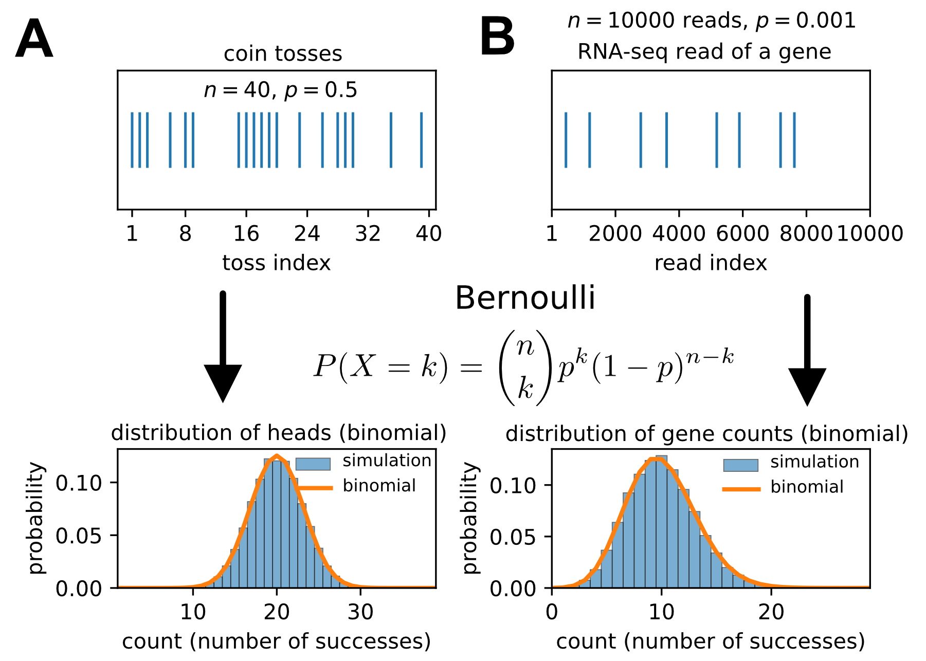
The coin-toss model introduced earlier illustrates this behavior. Each toss represents a single random event with two possible outcomes, occurring with probabilities \(p\) and \(1-p\). When many repeated coin-toss experiments are performed, the total number of heads obtained is not fixed. Instead, it fluctuates from experiment to experiment, following a probability distribution. Mathematically, each toss is described by a Bernoulli distribution, and the total number of heads follows a binomial distribution (Fig. 15.1A).
Strikingly, many biological counting experiments follow the same logic. Each molecule, cell, or genetic element represents a potential trial analogous to a coin toss: it is either detected or not, mutated or not, sequenced or not.
As a concrete example, consider a typical RNA-seq experiment in which thousands or millions of sequencing reads are generated from a pool of transcripts encoding a lot of different genes. Each read can be viewed as a random draw from this pool. Focusing on a single gene, each draw has some probability of originating from that gene. The observed read count therefore reflects the outcome of many such random trials, a Bernoulli process (Fig. 15.1B).
In principle, many biological counting experiments (such as RNA sequencing) sample molecules from a finite pool without replacement. However, in most omics experiments, the total number of molecules greatly exceeds the number of reads. Removing one molecule has a negligible effect on the remaining pool. In this limit, sampling without replacement is well approximated by independent Bernoulli trials. Note that this can be different in single-cell methods like single-cell RNA-Seq where available reads be very low.
15.2 From binomial to Poisson: rare events and large numbers
In most biological systems, individual events occur with very small probabilities (in contrast to a coin flip) but have many opportunities to occur. Consider again RNA-seq as an example. In a pool of transcripts from thousands of genes, the probability that a given read originates from one specific gene is typically very small. However, many millions of reads are analyzed to assemble a useful picture of gene expression. This logic applies similarly to proteomics spectral counts, barcode sequencing, and other high-throughput assays (see box below).
Many modern high-throughput counting experiments share the same basic structure: individual events are rare, but the number of opportunities for these events is very large.
Common examples include:
each DNA snippet has a small probability of being sequenced, but millions of molecules are sampled,
each transcript has a small probability of being detected in single-cell assays, but thousands of cells are measured,
each peptide has a small probability of being identified in mass spectrometry, but large peptide pools are analyzed,
each barcode has a small probability of being sampled in lineage-tracking experiments, but many lineages are tracked,
each cell division has a small probability of mutation, but many divisions are observed.
In all of these cases, measurements arise from many independent trials with a small success probability \(p\) and a large number of trials \(n\), leading to a finite expected count \(\lambda = np\).
This combination of rare events and many opportunities naturally gives rise to Poisson statistics.
In such scenarios, large numbers of trials with rare successes, the number of counts obtained for a single element is well described by Poisson statistics: \[P(X = k) = \frac{\lambda^k e^{-\lambda}}{k!}, \qquad k = 0,1,2,\dots\] where \(\lambda\) is the expected number of events. For example, when analyzing \(10^6\) sequencing reads, if a gene contributes on average about 1000 reads, then \(\lambda \approx 1000\).
Importantly, this formula naturally arises as a limit of the binomial distribution (see box). To consider counting statistics we thus specifically focus on the Poisson distribution in the following.
The Poisson distribution arises as a limiting case of the binomial distribution.
For a binomial process with \(n\) trials and success probability \(p\), \[P(X = k) = \binom{n}{k} p^k (1-p)^{n-k}.\]
Now consider the limit where \[n \to \infty, \qquad p \to 0, \qquad \lambda = np \ \text{is fixed}.\]
In this regime, we can approximate: \[\binom{n}{k} \approx \frac{n^k}{k!}, \qquad p^k = \left(\frac{\lambda}{n}\right)^k, \qquad (1-p)^n \approx e^{-\lambda}.\]
Substituting, \[P(X = k) \approx \frac{n^k}{k!} \left(\frac{\lambda}{n}\right)^k e^{-\lambda} = \frac{\lambda^k e^{-\lambda}}{k!}.\]
This is exactly the Poisson distribution.
15.3 Mean–variance relationships in counting data
A defining feature of the Poisson distribution is that it is fully determined by a single parameter, the expected number of events \(\lambda\). Once \(\lambda\) is specified, the entire distribution is fixed.
What then is the standard deviation or variance of the Poisson distribution? It is given by the same parameter: For a Poisson-distributed random variable \(X\), the mean and variance are equal: \[\mathbb{E}[X] = \mathrm{Var}(X) = \lambda.\]
This relation means that the variation of this distribution is substantial. Specficically:
Low-count measurements are dominated by statistical noise,
relative uncertainty is largest for rare events (small \(\lambda\),
higher counts (larger \(\lambda\)) are more precise but still noisy,
distributions become approximately Gaussian at large \(\lambda\).
These properties are illustrated in Fig. 15.2.
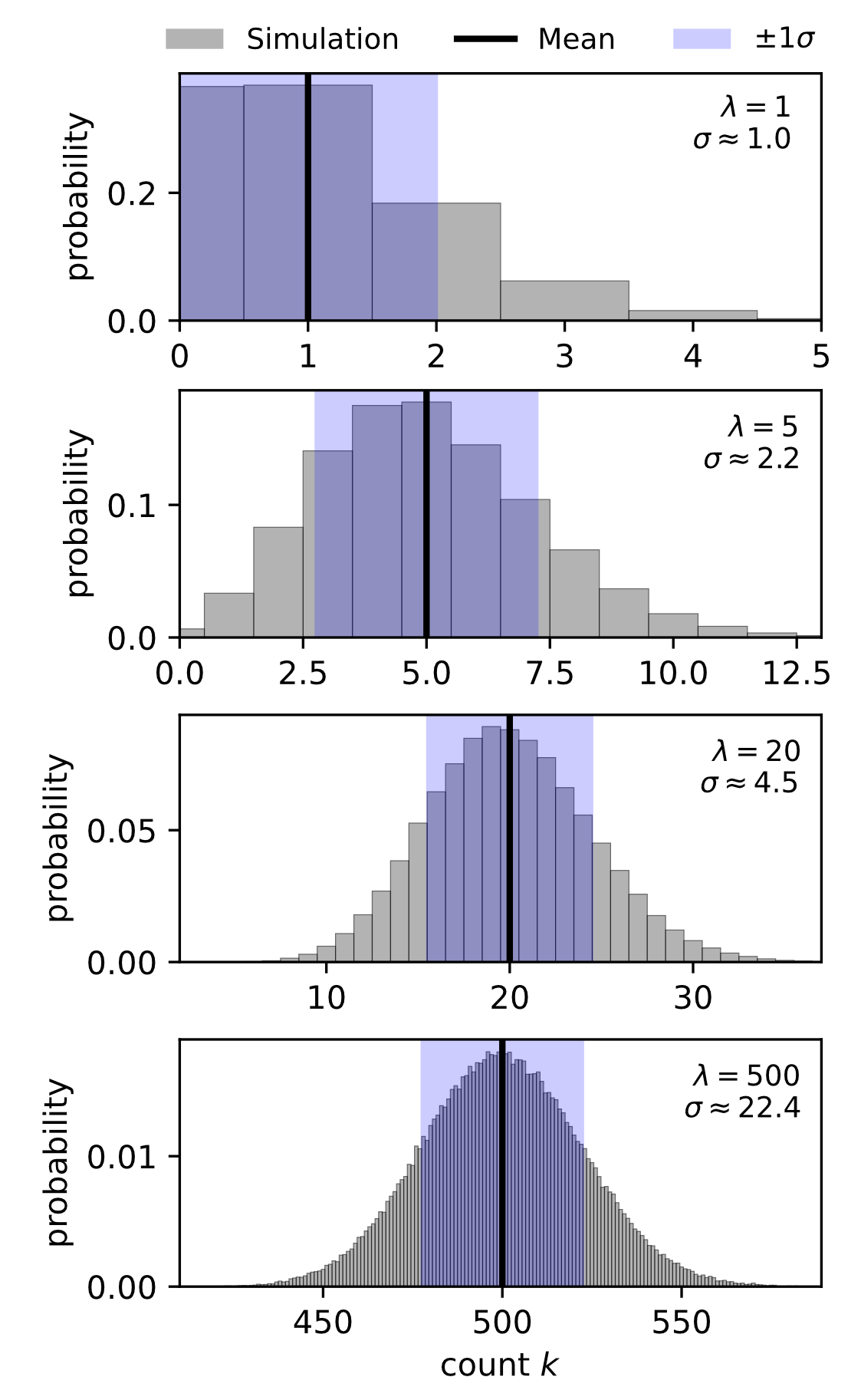
A useful RNA-seq intuition is to compare two genes with different expression levels. Suppose one gene has \(\lambda=5\) reads per sample, while another has \(\lambda=500\). For the lowly expressed gene, the standard deviation is \(\sqrt{5}\approx2.2\), comparable to the mean. For the highly expressed gene, the standard deviation is \(\sqrt{500}\approx22\), which is small relative to the mean. Thus, highly expressed genes are intrinsically easier to quantify than lowly expressed genes.
15.4 Biological noise, overdispersion, and negative binomial models
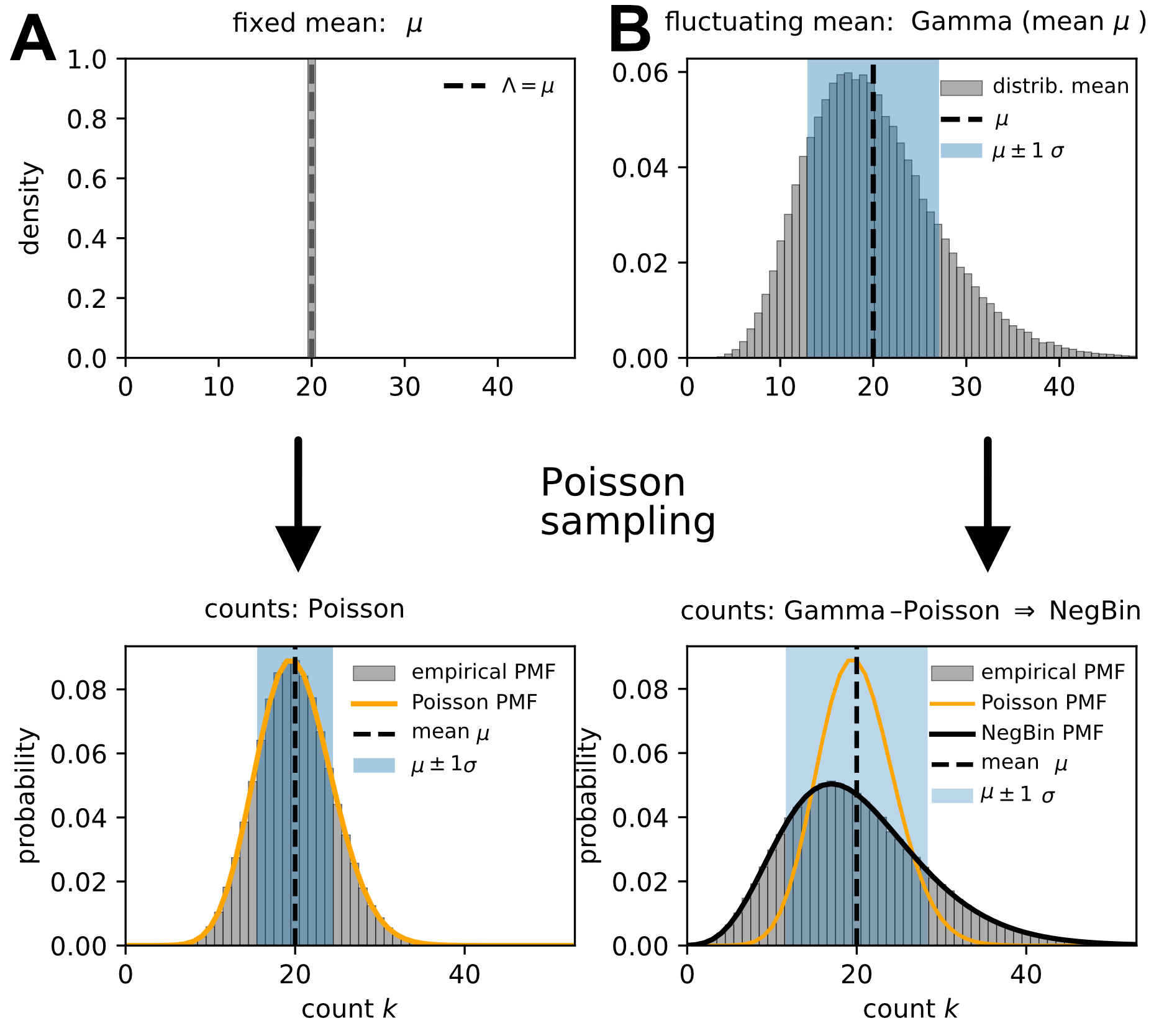
In contrast to many continuous measurements, counting noise cannot be separated from the signal itself. The Poisson distribution provides a natural baseline model for this sampling noise. However, real biological data often exhibit substantially more variability than predicted by Poisson statistics. That is, the observed variance is commonly higher than the mean: \[\mathrm{Var}(X) > \mathbb{E}[X].\] This phenomenon is known as overdispersion. Overdispersion reflects additional sources of variation such as cell-to-cell heterogeneity, bursty gene expression, unobserved regulatory fluctuations, and technical variability. As a result, Poisson models provide a useful lower bound on measurement noise, but it is often necessary to go beyond the Poisson model and account for additional variability.
A common way to account for overdispersion is the negative binomial distribution. It arises naturally when a Poisson process is combined with a fluctuating (Gamma-distributed) expectation value \(\lambda\). This mechanism is illustrated in Fig. 15.3. For a fixed mean \(\lambda\), counting noise is described by a Poisson process (Fig. 15.3A), whereas for a fluctuating mean, the resulting count distribution follows a negative binomial model (Fig. 15.3B).
For the negative binomial distribution, the variance is given by \[\mathrm{Var}(X) = \mu + \frac{\mu^2}{\theta},\] where \(\theta\) is the dispersion parameter that quantifies the additional variability relative to a Poisson process. In the limit \(\theta \to \infty\), the negative binomial distribution reduces to the Poisson distribution.
Historically, the negative binomial distribution was introduced to describe how many failures occur before a fixed number of successes in repeated Bernoulli trials. Mathematically, the same distribution also arises from a binomial expansion with a negative exponent (Taylor series expansion of \((1-p)^{-r}\)), hence the name.
State-of-the-art methods for analyzing omics data build directly on these basic principles of counting statistics, with the negative binomial distribution as a starting point, as we will discuss in Section ??.
In the following section, we will also examine the classic fluctuation test of Luria and Delbrück, a highly influential experiment that introduced rigorous statistical reasoning into molecular biology.